

Attention computes a weighted aggregation of value vectors, using compatibility scores between a query and the available keys. In standard scaled dot-product attention, the scores are scaled, masked and normalized with softmax before weighting the values. A token's representation can therefore incorporate information from other allowed positions.
The calculation has four stages:
- Project input representations into queries, keys and values.
- Calculate query–key compatibility scores.
- Mask disallowed pairs and normalize each query's scores.
- Compute the weighted sum of values for each query.
Learn the equation first, then distinguish three engineering decisions: which positions may interact, how the kernel executes those interactions, and what state the serving system caches. These decisions affect correctness, capacity and cost in different ways.
This chapter zooms into the attention portions of LLM Fundamentals. Tokenization Deep Dive explains where the positions come from. Transformer Architecture shows how attention fits beside feed-forward networks, residual paths, normalization, and position information.
Table of Contents
- The core idea
- Queries, keys, and values
- Scaled dot-product attention
- Tensor shapes
- Masks
- Self-attention and cross-attention
- Multi-head attention
- MHA, GQA, and MQA
- What attention weights do and do not explain
- Why dense attention is quadratic
- Sparse, windowed, and linear alternatives
- FlashAttention
- Prefill and decode
- The K/V cache
- Paged and prefix caching
- Other cache-reduction designs
- Practical system-design reasoning
- Common misunderstandings
- Interview questions
- Compact reference
- Engineering references
1. The Core Idea
Consider:
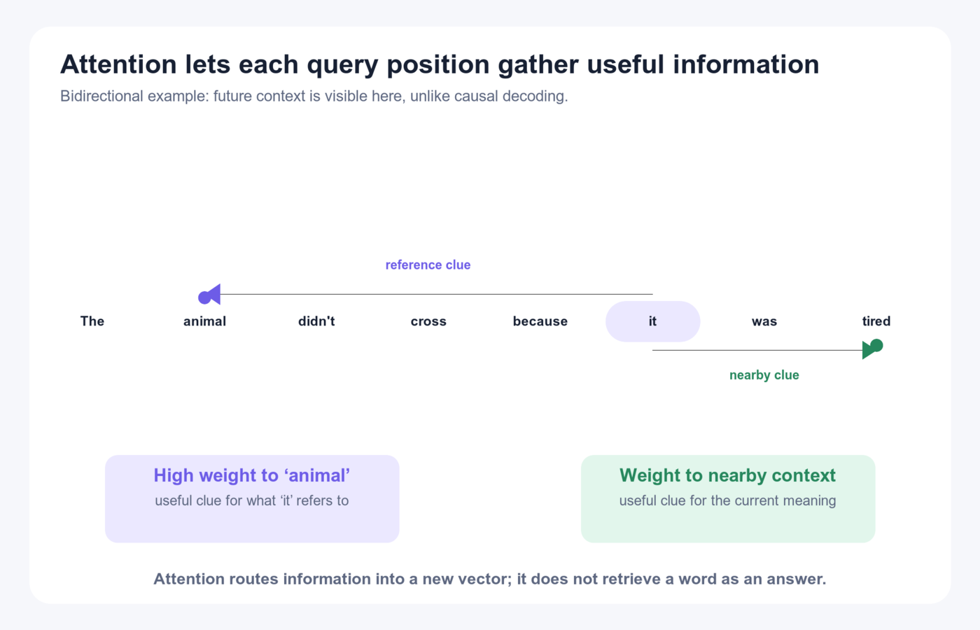
The animal did not cross the road because it was tired.
To build a useful vector for it, the model may use information from animal. Attention provides a direct path between those positions. The diagram illustrates bidirectional attention: it can also use the later word tired. A causal decoder processing it cannot read that future word. The arrows are illustrative weights, not a measured explanation of a particular model.
For one query position, attention produces a weighted combination:
new information
  = weight₁ × value₁
  + weight₂ × value₂
  + ...
  + weightₜ × valueₜ
The weights are non-negative and sum to 1 after softmax, provided the row has at least one finite, allowed score. This describes weights before attention dropout; dropout can change their sum. Masked positions have weight 0. A large weight means that a value contributes strongly in that head, layer, and forward pass.
Attention moves vectors, not words
If it attends to animal, the model does not copy the string animal into a secret text slot. It blends a learned value vector derived from that position. The result is another vector.
Every position does this
During a normal full-sequence attention call, each query position builds its own row of weights over allowed key positions. That creates a matrix:
rows    = query positions
columns = key positions
cell    = how strongly this query uses this key's value
This pairwise matrix is the source of both attention's flexibility and its sequence-length cost.
2. Queries, Keys, and Values
Each attention layer contains learned projection matrices. In a simple single-head notation:
Q = X W_Q
K = X W_K
V = X W_V
X contains the incoming hidden vector at each position.
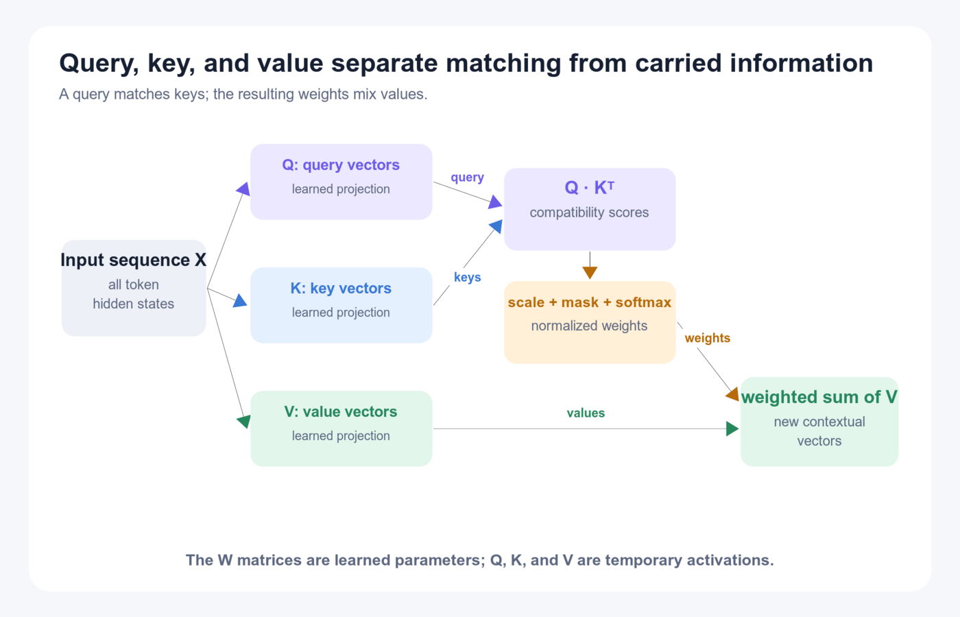
Query: the representation used to score candidate keys
Each query vector comes from the position whose output is being computed. Its dot products with keys determine their compatibility scores.
Key: the representation matched against a query
The key is used for matching. A query and key with a high dot product are compatible in that head's learned space.
Value: the representation included in the weighted sum
The value carries the content that is actually blended into the result.
Matching and carrying are separated
Keys are used to calculate weights. Values are mixed by those weights. The separation lets a position advertise one matching signature while contributing another learned representation.
Parameters versus activations
This distinction is essential:
| Object | Type | Lifetime |
|---|---|---|
W_Q, W_K, W_V, W_O |
Learned model parameters | Stored in the checkpoint; fixed during ordinary inference |
Q, K, V |
Runtime activations | Computed from the current input at each layer |
| Attention scores and weights | Runtime activations | Computed for the current attention call |
Saying “Q, K, and V are learned weights” is imprecise. The projection matrices are learned weights; the projected Q/K/V tensors depend on the current hidden states.
3. Scaled Dot-Product Attention
The standard equation is:
Attention(Q, K, V)
  = softmax((QKᵀ / √d_head) + mask) V
Read it from left to right.
Step 1: compare queries with keys
scores = QKᵀ
Every query vector takes a dot product with every allowed key vector.
Toy example for one query:
query q = [1, 2]

key k₁ = [2, 0]   q · k₁ = 2
key k₂ = [0, 1]   q · k₂ = 2
key k₃ = [1, 1]   q · k₃ = 3
Before masking and softmax, k₃ has the highest match score.
Step 2: divide by the square root of head width
scaled_scores = scores / √d_head
Under the simplifying assumption that query/key components are independent, zero-mean and unit-variance, the dot product has variance d_head. Large score magnitudes can saturate softmax and reduce useful gradients. Learned activations need not satisfy these assumptions exactly; they motivate the scale. Unit variance per component is not unit vector length: independently sampled unit-length vectors have different dot-product variance.
Dividing by √d_head keeps the score scale more controlled.
The denominator uses the query/key head width, not necessarily the model's full hidden width.
Step 3: apply the mask
An additive mask assigns 0 to allowed positions and −∞ to disallowed positions:
masked_score = −∞
After softmax, blocked weights become zero when at least one allowed score is finite. A finite negative sentinel only approximates this. A row of only −∞ has no ordinary softmax distribution; a kernel may define a special zero-output convention, but that behavior must be checked. Do not repair an all-blocked row by accidentally making forbidden tokens visible.
Step 4: softmax each query row
For scores s₁ ... sₜ:
weightᵢ = exp(sᵢ) / Σⱼ exp(sⱼ)
Numerically stable implementations subtract the row maximum before exponentiation. This changes none of the resulting probabilities but prevents overflow.
Step 5: mix values
output = weights V
Each output row is the weighted sum of value rows for one query.
Complete numeric example
Continue the same query and keys above, with no blocked positions:
raw scores    = [2, 2, 3]
scaled scores = [1.414214, 1.414214, 2.121320]
weights       ≈ [0.248255, 0.248255, 0.503490]

v₁ = [1, 0], v₂ = [0, 2], v₃ = [2, 1]
output ≈ 0.248255[1,0] + 0.248255[0,2] + 0.503490[2,1]
       ≈ [1.255235, 1.000000]
Blocking the third key instead gives weights [0.5, 0.5, 0] and output [0.5, 1]. The result is a new vector, not the index of the largest weight.
4. Tensor Shapes
Let:
B       = batch size
T       = sequence length
d_model = hidden width
H       = number of query heads
d_head  = width per head
For conventional multi-head attention with equal query/key/value head widths and H × d_head = d_model:
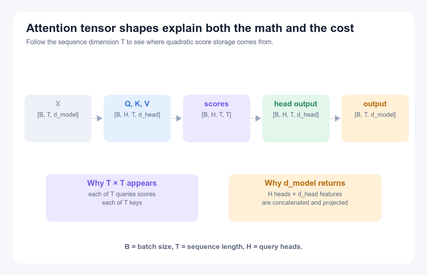
X:             [B, T, d_model]

Q, K, V:       [B, H, T, d_head]

Kᵀ:            [B, H, d_head, T]

QKᵀ:           [B, H, T, T]

softmax(...)V: [B, H, T, d_head]

concatenate:   [B, T, H × d_head]

output W_O:    [B, T, d_model]
Where T × T comes from
There are T query positions, and each scores T key positions. The score tensor therefore contains T² cells per head and batch item before masking or specialized sparse execution.
Decoder-only decode shape
During one cached decode step, the new query length is often 1 while the key/value length is the full cached context T:
Q:      [B, H_q, 1, d_head]
K/V:    [B, H_kv, T, d_head]
scores: [B, H_q, 1, T]
That rectangular 1 × T problem behaves differently on hardware from square prefill attention. Query and key widths must match for their dot product; value width may differ. Some architectures also choose H × d_head ≠ d_model and project back to the residual width. Read the actual model configuration rather than inferring every dimension from the hidden size.
Cross-attention shape
With target length T_target and source length T_source:
QKᵀ: [B, H, T_target, T_source]
Attention is pairwise across the two sequences, not necessarily square.
5. Masks
A mask decides which query-key pairs are legal.
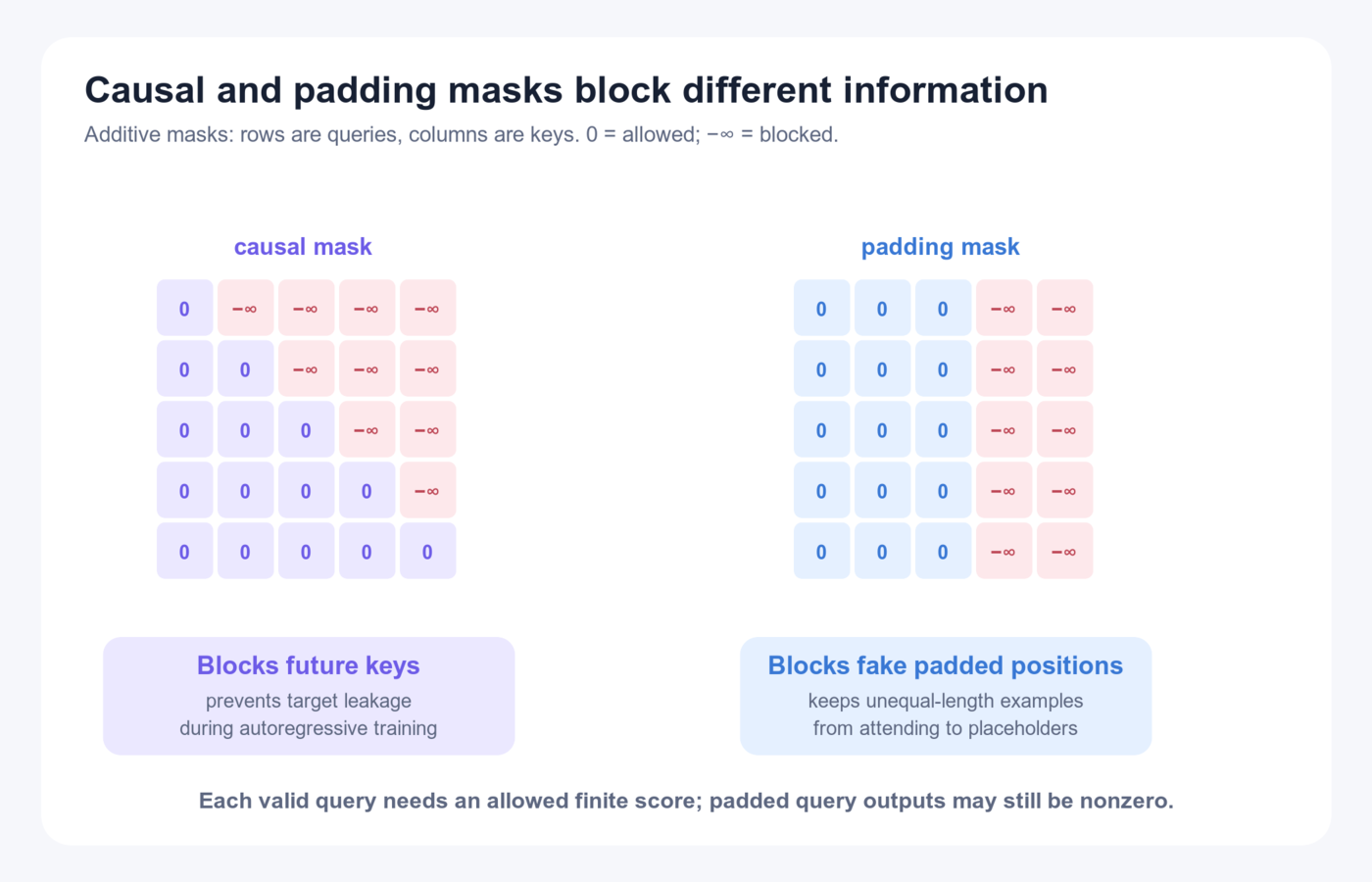
Causal mask
An autoregressive decoder must not use the token it is being trained to predict. The representation at input position i can read positions through i; its next-token target is at i + 1.
For four positions:
query 1 may read: 1
query 2 may read: 1, 2
query 3 may read: 1, 2, 3
query 4 may read: 1, 2, 3, 4
The allowed region is lower triangular for a full sequence whose query and key positions start together.
| Input position | Input token | Target predicted from that position |
|---|---|---|
| 0 | BOS |
The |
| 1 | The |
cat |
| 2 | cat |
slept |
Reading the current input is valid because the labels are shifted. Reading the next input would leak the target.
This lets training process all target positions in parallel while preserving the next-token task. Position 3 can compute at the same time as position 2, but its mask still hides positions 4 and beyond.
Padding mask
Examples in one batch often have different lengths. Shorter sequences may be padded to a common tensor length:
[real, real, real, PAD, PAD]
A padding mask stops queries from treating placeholder keys as content. It does not necessarily make padded query outputs zero: those queries can still attend to real keys. Exclude padded targets from the loss and discard padded outputs as appropriate.
Segment or document masks
Packed training or inference can place several independent sequences in one physical tensor. A block-diagonal document mask can prevent tokens from reading across example boundaries.
Additive and Boolean masks
Check the exact interface; Boolean conventions differ even inside one framework.
| Interface, checked September 24, 2026 | Boolean True means |
|---|---|
PyTorch 2.14 scaled_dot_product_attention(..., attn_mask=...) |
Pair is allowed |
PyTorch 2.14 MultiheadAttention(..., attn_mask=...) |
Pair is blocked |
PyTorch 2.14 MultiheadAttention(..., key_padding_mask=...) |
Key is ignored |
Float masks are added to scores. In functional SDPA, explicitly use dropout_p=0.0 during evaluation; the function applies the supplied dropout probability regardless of the calling module's evaluation state. See SDPA and MultiheadAttention.
Cached decoding: align positions, not just matrix corners
Suppose three positions are cached and two new positions are processed together. The combined keys have positions 0–4; the new queries have positions 3,4:
                       key position
                     0  1  2  3  4
query at position 3  1  1  1  1  0
query at position 4  1  1  1  1  1

1 = allowed, 0 = blocked
A plain upper-left triangular 2 × 5 mask is wrong here. PyTorch SDPA's non-square is_causal=True uses upper-left alignment; FlashAttention's documented causal behavior since version 2.1 uses lower-right alignment. Do not transfer a flag's meaning between interfaces. Use an explicit position-aware mask or the appropriate causal bias, and verify against the kernel contract.
This standard-library example constructs allowed pairs for one contiguous, unpadded sequence. past_length counts valid cached positions, not allocated block capacity. It is a reference for inspecting masks, not an efficient tensor implementation:
def causal_allowed(past_length, query_length):
    """Rows are newly appended queries; columns include past and new keys."""
    if type(past_length) is not int or past_length < 0:
        raise ValueError("past_length must be a non-negative integer")
    if type(query_length) is not int or query_length <= 0:
        raise ValueError("query_length must be a positive integer")
    key_length = past_length + query_length
    return [
        [key <= past_length + row for key in range(key_length)]
        for row in range(query_length)
    ]

assert causal_allowed(3, 2) == [
    [True, True, True, True, False],
    [True, True, True, True, True],
]
assert causal_allowed(4, 1) == [[True] * 5]
For left padding, packed documents, sliding windows or noncontiguous positions, combine causal position comparisons with valid-key and segment masks; a single length offset is insufficient. When passing a complete explicit mask to SDPA, leave is_causal=False. Test full-prefill outputs against cached one-token and chunked outputs within the chosen numerical tolerance.
6. Self-Attention and Cross-Attention
Self-attention
Queries, keys, and values are projected from the same sequence of hidden states:
Q = XW_Q
K = XW_K
V = XW_V
The mask determines whether the sequence is bidirectional, causal, windowed, or otherwise restricted.
Cross-attention
Queries come from one sequence; keys and values come from another:
Q = X_target W_Q
K = X_source W_K
V = X_source W_V
In an encoder-decoder translation model:
- the encoder builds source-language memory,
- the decoder state supplies queries,
- and cross-attention selects useful source values for each target position.
The Transformer Architecture chapter contains the complete encoder-decoder diagram, so it is not duplicated here.
Other uses
Cross-attention can connect:
- text queries to image features,
- generated audio states to text encodings,
- a diffusion model to conditioning embeddings,
- or a small set of learned latent queries to a large input.
The defining feature is the source of Q versus K/V, not the application name.
7. Multi-Head Attention
One attention calculation gives one learned matching space. Multi-head attention runs several in parallel.
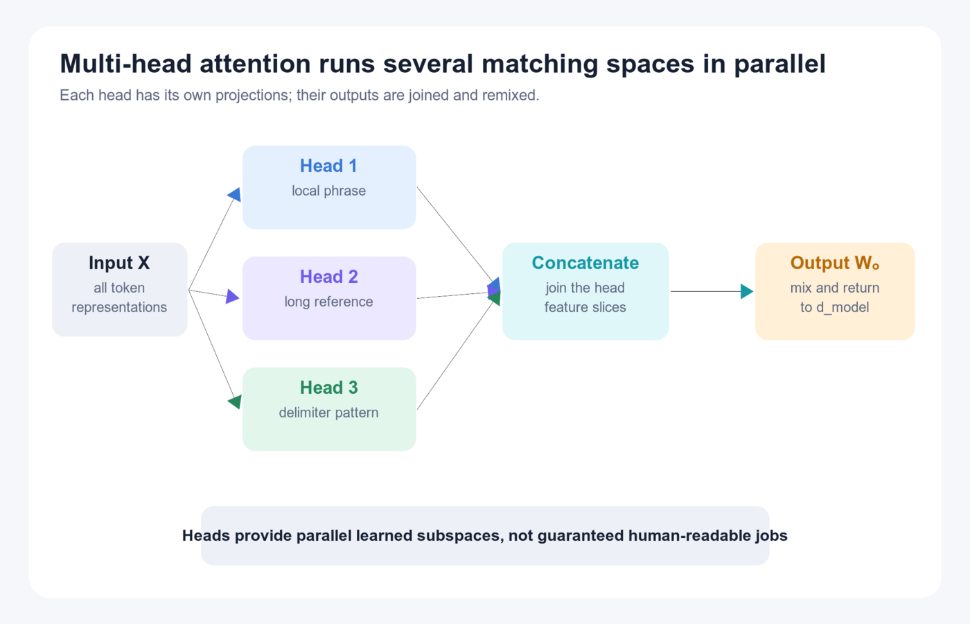
For each head h:
head_h = Attention(XW_Q^h, XW_K^h, XW_V^h)
Then:
MultiHead(X)
  = Concat(head₁, ..., head_H) W_O
Why several heads help
Each head has separate projections. That gives the layer several learned subspaces in which to compare and move information.
Different heads may exhibit:
- local positional patterns,
- delimiter behavior,
- copying behavior,
- syntactic or reference patterns,
- or distributed features that do not have a clean English label.
Head width
In a conventional design:
d_head = d_model / H
For d_model = 1024 and H = 16:
d_head = 64
The model still returns one d_model-wide vector after concatenation and W_O.
Heads are not an ensemble of full models
The heads share the surrounding layer, residual stream, training objective, and output projection. They are parallel feature pathways inside one operation, not independent voters with separate final predictions.
8. MHA, GQA, and MQA
Autoregressive serving stores keys and values for past positions. Reducing the number of K/V heads can shrink that cache.
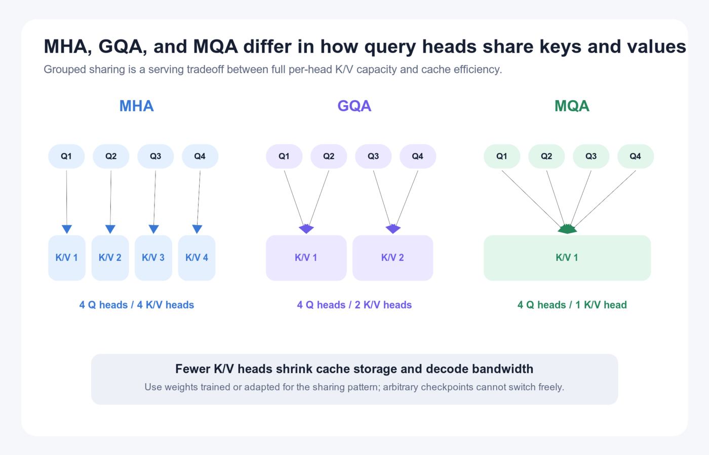
Multi-Head Attention (MHA)
Each query head has its own K/V head:
H_q = H_kv
This provides full per-head K/V capacity and the largest cache among the three patterns.
Multi-Query Attention (MQA)
All query heads share one K/V head:
H_kv = 1
Cache storage and K/V memory traffic fall substantially. The stronger sharing constraint can affect model quality, so it is an architectural and training choice.
Grouped-Query Attention (GQA)
Groups of query heads share K/V heads:
1 < H_kv < H_q
Example:
32 query heads
8 K/V heads
4 query heads share each K/V head
GQA occupies the middle between MHA and MQA.
Not a transparent runtime switch
You cannot usually take arbitrary MHA weights, set a serving flag to MQA, and expect identical behavior. The head shapes and learned parameters differ. Conversion methods require adaptation or training.
Storage reduction
Holding other dimensions fixed, K/V-cache storage scales with H_kv. Moving from 32 K/V heads to 8 reduces this part of cache storage by a factor of four.
That is a structural ratio, not a promise that total request memory or end-to-end latency improves by exactly four. Model weights, activations, allocator overhead, batching, and other kernels still matter.
9. What Attention Weights Do and Do Not Explain
An attention heatmap can be useful for inspection:
            key position
           The  cat  slept
query The   .80  .10   .10
query cat   .35  .55   .10
query slept .15  .45   .40
This illustrative bidirectional heatmap shows one head's normalized routing weights for one layer and input. A causal version would have zero weights above its diagonal.
What a high weight supports
A high weight says:
In this calculation, this query used a relatively large fraction of that key position's value.
What it does not prove
It does not by itself prove:
- a human-readable causal explanation,
- that the attended token determined the final answer,
- that the value vector contains only the visible word's meaning,
- that another head or layer did the same thing,
- or that zeroing this edge would produce the expected counterfactual.
Why the interpretation is limited
The final prediction depends on:
- value vectors, not weights alone,
- multiple heads,
- output projections,
- residual streams,
- feed-forward networks,
- every later layer,
- and the decoding decision.
Two positions can receive equal weights but contribute very different vectors. A small weight on a large or directionally important value can matter.
Better analysis
Combine attention views with:
- activation and attribution methods,
- ablation or patching experiments,
- counterfactual inputs,
- and end-to-end behavioral tests.
Use heatmaps as evidence about routing, not as a complete explanation of reasoning.
10. Why Dense Attention Is Quadratic
For T query positions and T key positions, dense self-attention scores:
T × T = T² position pairs per head
Doubling sequence length from T to 2T creates:
(2T)² = 4T²
four times as many pair scores.
More precise operation picture
Computing QKᵀ uses roughly:
O(T² d_head)
per head, and mixing weights with V has the same broad order. The score/weight intermediate has:
O(T²)
elements per head.
Linear projections and feed-forward networks have their own costs. Saying “the entire Transformer is O(T²)” is a shortcut about the dominating attention term at long sequence lengths, not a complete runtime model for every shape.
A mask does not automatically save work
A causal mask blocks roughly half of a square score matrix semantically. A dense implementation may still compute or allocate a full matrix before applying that mask.
To reduce work, the kernel must exploit the structure and skip blocked tiles.
Decode is rectangular
With a K/V cache, one new query attends to T cached positions:
1 × T scores per head for that decode step
One step grows linearly with cached context length. Generating many tokens repeats that work serially while the cache grows.
11. Sparse, Windowed, and Linear Alternatives
Not every task needs every position to interact directly with every other position in every layer.
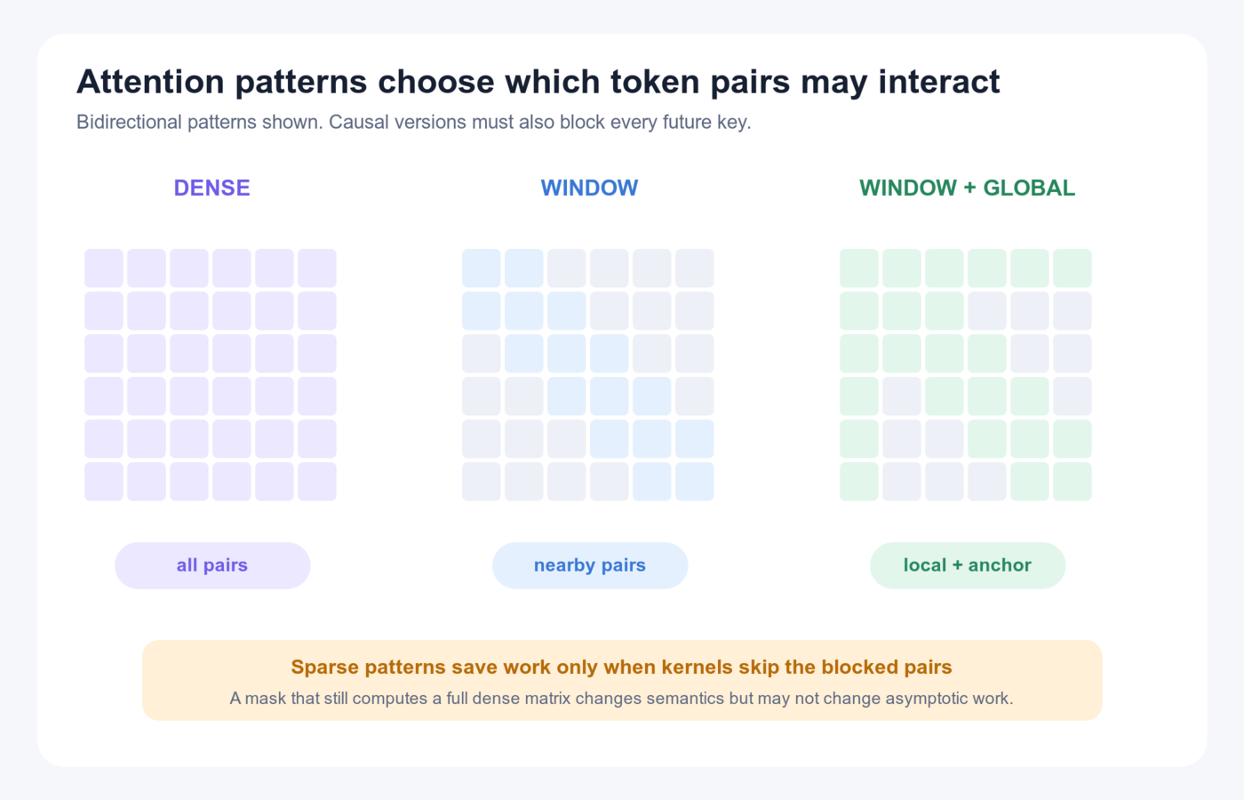
Sliding-window attention
Each query reads a fixed neighborhood of width w:
O(Tw) pair interactions
This is linear in T only while w stays fixed. Local context is cheap and direct. Information can travel farther through multiple layers, but a single layer cannot connect arbitrary distant positions.
Local plus global tokens
Most positions use a local window, while g global positions can read and be read broadly. Work is approximately O(T(w + g)) when kernels exploit the pattern; it is linear in T only for fixed w and g. The diagram is bidirectional. A causal variant must also block future reads, including through global positions and earlier layers.
Block-sparse attention
The sequence is divided into blocks, and only selected block pairs interact. Hardware-friendly block structure matters because irregular single-edge sparsity may save theoretical operations but execute poorly.
Dilated or strided patterns
Positions attend locally plus at regular gaps. That expands reach while keeping fewer connections.
Linear-attention families
Kernelized linear attention uses non-negative compatibility scores φ(q)ᵀφ(k) instead of the exponential dot-product kernel. For causal attention, define column feature vectors of width r:
Sₜ = Sₜ₋₁ + φ(kₜ) vₜᵀ       shape [r, d_value]
zₜ = zₜ₋₁ + φ(kₜ)            shape [r]
yₜᵀ = (φ(qₜ)ᵀ Sₜ) / (φ(qₜ)ᵀ zₜ)
Initialize both states to zero. The denominator is essential: writing only φ(Q)(φ(K)ᵀV) gives the numerator, not normalized attention. The original linear-Transformer example uses φ(x) = ELU(x) + 1. Guard against a zero or numerically tiny denominator using the implementation's specified policy.
State is r × d_value + r elements per head; attention work is O(T r d_value) excluding feature-map computation. It is linear in sequence length for fixed widths. This is exact for its chosen kernel, generally not exact softmax attention. Modern gated or delta-rule variants use different updates; do not assume this recurrence describes all linear-attention models. See Linear Transformers, equations 9–12.
Sparse semantics versus sparse execution
A sparse mask describes allowed edges. Speed arrives only when the runtime uses a kernel or compiler that avoids the blocked tiles efficiently. A dense fallback with a sparse-looking mask can preserve semantics while saving little work.
12. FlashAttention
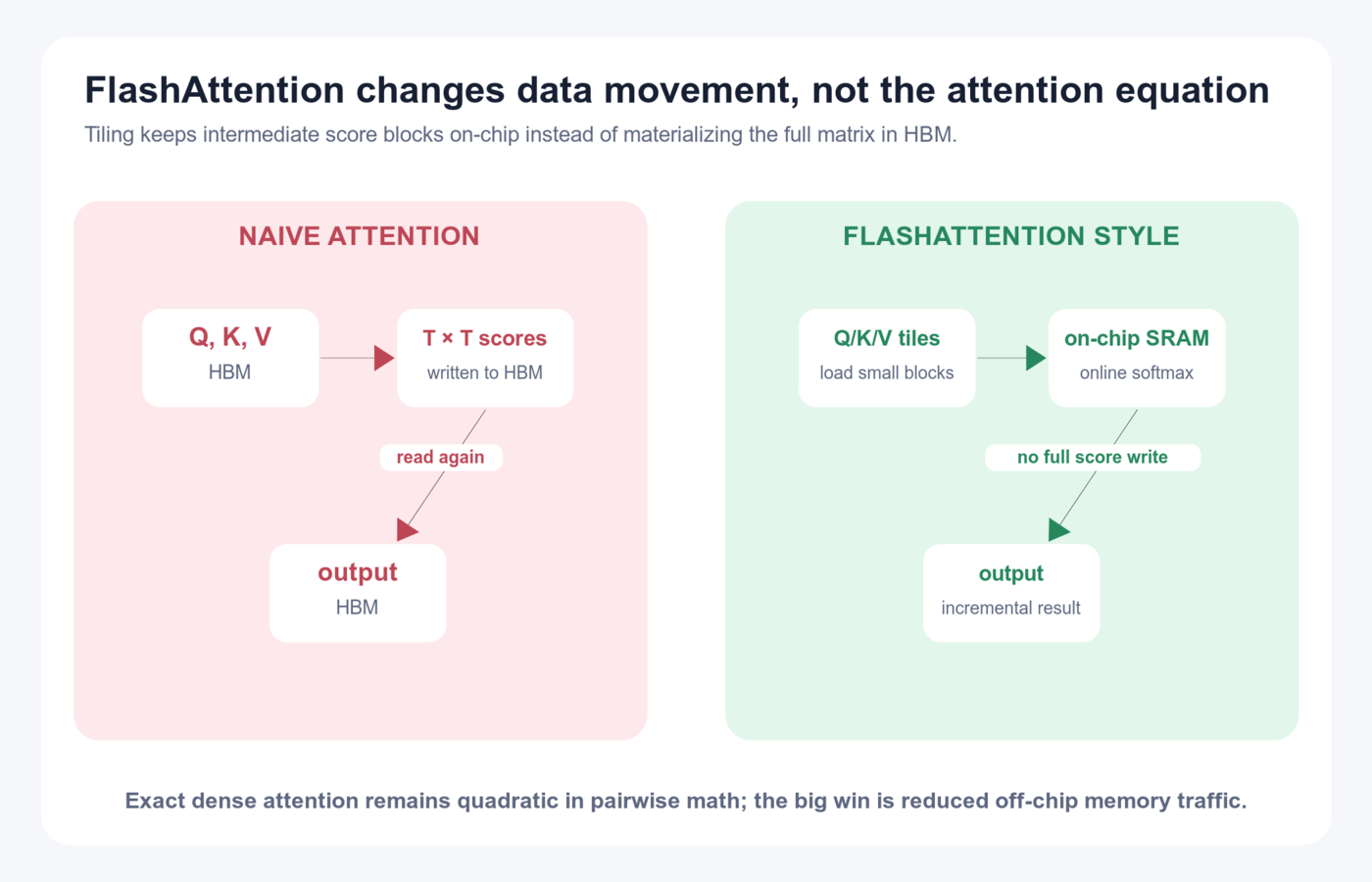
FlashAttention computes exact dense softmax attention while reducing expensive memory movement.
The hardware problem
Modern accelerators have a memory hierarchy:
- large off-chip high-bandwidth memory (HBM),
- much smaller and faster on-chip SRAM/register storage,
- and arithmetic units that can sit idle while data moves.
A naive attention implementation can:
- read Q and K,
- write the large score matrix to HBM,
- read it for softmax,
- write normalized weights,
- read them again to multiply V.
The repeated movement of T² intermediates can dominate.
Tiling and online softmax
A FlashAttention-style kernel:
- loads blocks of Q, K, and V that fit on chip,
- computes a score tile,
- updates a numerically stable running softmax,
- accumulates the corresponding output contribution,
- avoids storing the complete score/weight matrix in HBM.
The running maximum, normalization sum and accumulated output combine tiles exactly in real arithmetic. Floating-point operation order can still change numerical results. Lower-precision variants also introduce representation error; “exact attention” does not promise bitwise equality across kernels or formats.
What complexity changes?
For dense attention:
- pairwise arithmetic remains quadratic in sequence length,
- the attention equation is unchanged,
- but off-chip intermediate storage becomes linear with sequence length rather than materializing the full quadratic matrix,
- and reduced HBM traffic can make the kernel much faster.
So this statement is wrong:
FlashAttention makes dense attention
O(T)compute.
The better statement is:
FlashAttention keeps exact dense attention's quadratic pairwise math but reorganizes it to use much less off-chip memory traffic and intermediate storage.
Forward and backward passes
During training, saving every attention probability for backward propagation is expensive. FlashAttention can recompute selected tile results from compact saved statistics rather than store the whole matrix. Extra arithmetic can be cheaper than extra HBM traffic.
Versions and implementations
| Implementation family | Main distinction | Interview implication |
|---|---|---|
| FlashAttention-2 | Improved GPU work partitioning and parallelism | Check shapes and backend dispatch |
| FlashAttention-3 | Hopper-focused asynchronous execution | Hardware generation matters |
| FlashAttention-4 | CuTe DSL implementation targeting Hopper and Blackwell | Verify package, GPU, dtype and supported operations |
This snapshot was checked September 24, 2026 against the maintainers' implementation and the FlashAttention-4 paper. PyTorch 2.14's SDPA documentation lists FlashAttention-2 among its backends; installing a newer standalone package does not prove that SDPA dispatches to it. Inspect the actual kernel in a profiler. A correct fallback can still be slower.
A separate September 2026 low-precision FA4 implementation describes block-scaled MXFP8 forward/backward attention on Blackwell. Its published throughput and speedups apply to the measured training shapes and hardware. They do not establish the gain for a single-token decode workload or guarantee unchanged model quality.
13. Prefill and Decode
Autoregressive inference has two attention workloads.
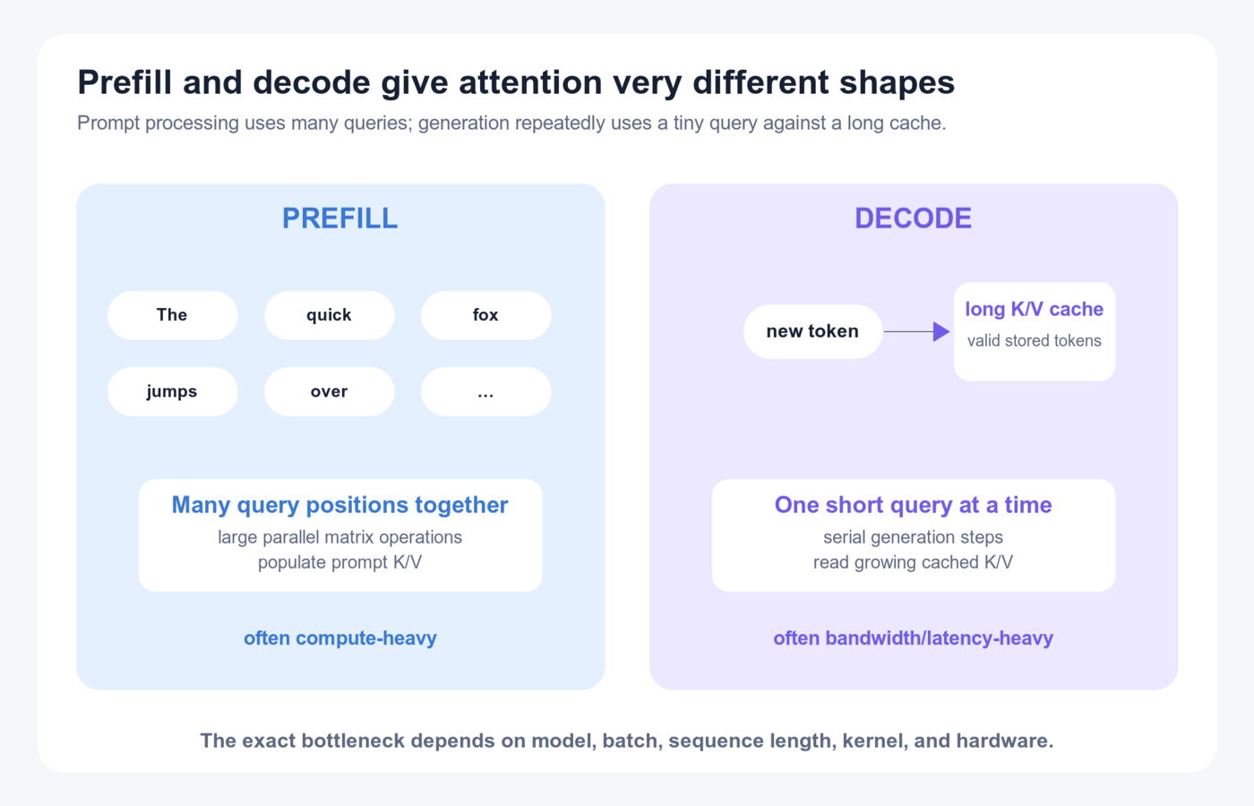
Prefill
The model processes the prompt positions:
query length ≈ prompt length
key/value length ≈ prompt length
The workload contains large matrix operations with substantial parallelism. Prefill produces:
- hidden states through all layers,
- prompt K/V entries for each attention layer,
- and logits for the first generated token.
Time to first token includes prefill plus surrounding scheduling and network work.
Decode
After selecting one new token:
query length = 1
key/value length = prompt + generated-so-far
The model must run another forward step before it can choose the next token. Generation is serial across token steps even though each step uses parallel hardware internally.
Decode often becomes sensitive to:
- K/V-cache reads,
- model-weight reads,
- batch size,
- scheduling,
- and per-step kernel launch/communication latency.
Avoid universal bottleneck labels
“Prefill is compute-bound and decode is memory-bound” is a useful first approximation, not a law. The outcome changes with model architecture, prompt length, batch size, speculative methods, quantization, parallelism, and hardware.
Measure time to first token and inter-token latency separately.
14. The K/V Cache
In ordinary causal inference, appending a token leaves earlier hidden states unchanged when the model, adapter, positional transformation and other computation settings stay fixed. Their keys and values remain valid. Changing weights or rescaling existing positions can invalidate that argument; bidirectional attention generally cannot reuse old states in the same way.
The K/V cache stores those activations.
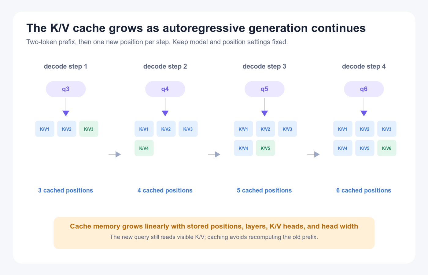
Without a cache
At every decode step, the model would recompute key and value projections for every previous position.
With a cache
At step t:
- compute the new position's Q, K, and V at the layer,
- append its K and V to the layer's cache,
- compare the new Q with cached keys,
- use the weights to mix cached values,
- continue through the rest of the layer and model.
What is cached?
For a conventional decoder, the persistent attention cache contains K and V tensors for stored positions at every cached layer, including the current position once appended. At the next step they are all prior positions.
It does not normally need to preserve earlier queries. Future tokens query the past; earlier queries are not reused to score a newly appended future key under causal decoding.
Storage formula
An approximate K/V-cache byte count is:
2
× layers
× stored_positions
× K/V_heads
× d_head
× bytes_per_element
× batch_or_active_sequences
The factor 2 is for keys plus values.
Example with deliberately small values:
2 × 4 layers × 100 positions × 2 K/V heads × 16 width × 2 bytes
= 51,200 bytes
Real runtimes add allocator metadata, block rounding, beam copies or sharing, and other state.
What caching removes
It removes repeated K/V projection and earlier-position forward work.
What caching does not remove
The new query still reads and scores relevant cached keys and mixes cached values. Its attention work grows with the context it can see.
Therefore this statement is misleading:
The K/V cache makes each decode step
O(1).
Projection work for the old prefix is avoided, but attention over a growing cached context is not constant.
15. Paged and Prefix Caching
These solve different problems and should not be collapsed into “the cache.”
Paged K/V-cache management
Serving many variable-length requests with large contiguous cache allocations wastes memory through fragmentation and reserved-but-unused space.
Paged attention systems divide K/V storage into blocks and map a request's logical positions to physical blocks. The analogy is virtual memory:
- blocks need not be contiguous,
- capacity can grow as tokens arrive,
- freed blocks can be reused,
- and shared prefixes can sometimes point to shared physical blocks.
Paged storage changes memory management. The attention kernel still has to locate and read the required K/V blocks.
Prefix caching
If requests share an identical serialized prefix, a server can reuse K/V already computed for that prefix:
same system prompt
+ same tool schema
+ same initial document
→ reusable prefix K/V
This can reduce repeated prefill work and time to first token.
Exact-match considerations
Prefix reuse normally depends on exact token IDs plus compatible:
- model checkpoint,
- adapter state,
- position handling,
- attention configuration,
- and the authorized trust scope for reuse.
Visually identical text that tokenizes differently is not the same prefix. Multimodal identity must also include the actual image/audio features or content hashes; equal placeholder token IDs do not identify equal media.
Security and isolation
Choose the allowed sharing boundary explicitly. In a tenant-isolated service, derive the cache scope from authenticated identity on the server; clients must not choose another tenant's scope. vLLM supports a cache_salt in prefix hashing: use a trusted scope-derived salt when enabling this mechanism, plus compatible model/media identity. Separation reduces cross-scope reuse and associated timing exposure; it is not a proof against every side channel. See vLLM prefix caching and isolation.
Application-level context caching
Some APIs expose cached-input pricing or explicit context-caching features. Those are product contracts around server-side reuse. Verify current provider semantics rather than assuming every “cache” stores the same tensors for the same duration.
16. Other Cache-Reduction Designs
Quantized K/V cache
Store cache entries in fewer bits and convert them to the computation format when needed.
Benefits can include:
- lower memory footprint,
- lower memory bandwidth,
- larger batch size or context.
Costs can include:
- quantization/dequantization work,
- numerical error,
- calibration or training requirements,
- and hardware-specific support.
Claims about quality and speed must name the precision format, model, workload, and hardware.
Sliding-window cache
If attention can see only the most recent w positions, older K/V may be dropped for those layers. Cache size can remain bounded by the window.
Some hybrid models combine local layers with occasional global or full-context layers. Their cache rules differ per layer.
MQA and GQA
Reducing K/V heads shrinks the per-position cache width. This was covered in section 8.
Multi-head Latent Attention (MLA)
MLA-style designs store a lower-dimensional latent representation from which the attention computation derives needed information. This aims to reduce cache storage and bandwidth through learned compression rather than only sharing K/V heads.
It introduces architectural details around projections and position encoding. Treat it as another design family with its own training and kernel requirements, not as a drop-in replacement that universally “wins.”
Eviction and compression
Research systems may keep selected tokens, merge cache entries, offload blocks to host memory, or evict low-value spans. These save accelerator memory by changing what information remains directly available or where it lives. Evaluate quality, transfer latency, and workload locality together.
Why MLA separates position from compressed content
In DeepSeek-V2's MLA, a small latent vector represents the content needed to recover keys and values. Without position-dependent rotations in that content path, projection matrices can be combined algebraically to avoid materializing all expanded cached vectors during attention. RoPE complicates this: its rotation depends on token position, so it cannot generally be absorbed into one fixed projection for every position.
The design therefore uses a decoupled positional path. A content score comes from compressed representations; an additional query/key component carries RoPE position information. Their contributions form the attention score. The cache retains the compressed content plus the required positional key information. This explains both the memory benefit and why “just compress K/V” leaves out part of the mechanism. Exact execution and speed depend on kernels; a smaller cache alone does not prove lower latency. See the DeepSeek-V2 architecture, section 2.1.3.
Recall check: What prevents us from absorbing ordinary RoPE into the same fixed projection? The rotation changes with position. What is the repair? Keep a separate positional component alongside the compressed content.
17. Practical System-Design Reasoning
Capacity equation
A simplified serving memory budget is:
accelerator memory
  ≈ model weights
  + active K/V caches
  + temporary activations/workspaces
  + runtime and communication buffers
Longer contexts increase per-request cache. Higher concurrency multiplies active caches. Lower-precision weights do not automatically solve K/V pressure.
Latency metrics
Separate:
- time to first token (TTFT): queueing + prefill + first-token selection,
- inter-token latency (ITL): delay between generated tokens,
- tokens per second per request: user-perceived stream rate,
- aggregate throughput: tokens processed across all requests.
Optimizing one can hurt another. Waiting to form a larger batch can improve aggregate throughput while increasing queueing latency.
Continuous batching
Requests enter and leave at different times. A serving scheduler can combine active decode steps and insert new prefill work without waiting for every sequence in a static batch to finish.
The scheduler must balance:
- prefill work versus decode deadlines,
- fairness,
- K/V capacity,
- maximum batch tokens,
- and latency service levels.
Model choice
When context and concurrency dominate, inspect:
- K/V-head count,
- head width and layer count,
- cache dtype,
- local versus global layers,
- kernel availability,
- and maximum supported batch/sequence shapes.
Parameter count alone does not determine serving memory.
Measure realistic shapes
Benchmarks should include distributions of:
- prompt length,
- output length,
- batch/concurrency,
- prefix-cache hit rate,
- adapter or model variants,
- and hardware topology.
One square-attention microbenchmark cannot predict mixed production traffic.
Worked interview: increase a private assistant from 16K to 32K context
Prompt: A private document assistant serves several tenants. Its context limit must grow from 16,384 to 32,768 tokens. Design the attention-serving changes without silently weakening isolation or overwhelming the fleet. These are interview assumptions, not a report of Learnastra traffic or a vendor benchmark.
1. Define functional requirements
- Accept authenticated chat requests using one pinned model release that supports the required context length.
- Stream output and return a clear overload or context-limit response when the request cannot be admitted.
- Budget the combined input and output within 32,768 tokens; for example, 31,744 input tokens plus 1,024 reserved output tokens.
- Reuse exact prefixes only within the authorized sharing scope and compatible model/adapter/position configuration.
- Release request cache blocks on completion, cancellation or expiry; preserve only explicitly eligible prefix blocks under the retention policy.
2. Agree on non-functional requirements
- Peak load: 60 simultaneously active requests. Measure arrival rate and output-length distribution before sizing throughput.
- Proposed latency targets: p95 TTFT below two seconds and p95 ITL below 80 ms, measured separately by input-length band. Validate whether 32K prompts can meet the TTFT target; negotiate a separate long-input target if necessary.
- Availability target: 99.9% of eligible requests successfully complete within the agreed service deadline, with overload counted according to the published SLO.
- Isolation: no reuse of private prefix state across unauthorized scopes; no prompt text in ordinary metrics or cache-debug logs.
- Quality: preserve the agreed task-success threshold across retrieval position, long documents and adversarial inputs; faster kernels must not silently change the selected model or attention pattern.
- Budget: compare full monthly operating cost and cost per successful request, including spare capacity and human operations.
3. Begin with a simple design and expose its limits
Start with a gateway, one queue and a model server using dense causal attention and a contiguous per-request K/V buffer. It is easy to inspect, but increasing the configured context limit alone creates several failures:
| Failure | Cause | Repair | Cost or limitation |
|---|---|---|---|
| Prefill runs out of memory | Materialized square score tensors grow fourfold | Use a supported tiled attention kernel | Still quadratic pairwise computation; verify dispatch |
| Too many long requests exhaust K/V memory | Per-request cache doubles | Admit by reserved token blocks and apply backpressure | Some requests wait or receive overload responses |
| Short streams pause behind large prompts | Unbounded prefill work competes with decode | Chunk prefill and schedule against decode deadlines | Scheduler complexity; prompt throughput can fall |
| Cached outputs differ from full prefill | Wrong query positions, mask alignment or valid lengths | Compare both paths using deterministic reference inputs | Extra correctness checks, not a speed optimization |
| A private prefix affects another tenant's latency | Cache identity omits trusted scope | Partition reuse by authenticated scope | Lower hit rate and more duplicated state |
| Quality falls after a window/precision change | Optimization changes retained information or numerical representation | Keep the original path, run task evaluations and canary the change | More temporary capacity; rollback must remain available |
4. Calculate memory before buying capacity
Assume a hypothetical GQA decoder has 32 full-attention layers, 32 query heads, eight K/V heads, head width 128 and BF16 cache values. Its per-position K/V storage is:
2 × 32 × 8 × 128 × 2 bytes = 131,072 bytes = 128 KiB
| Quantity | 16,384 positions | 32,768 positions |
|---|---|---|
| K/V per fully reserved request | 2 GiB | 4 GiB |
| One materialized BF16 score matrix per head | 512 MiB | 2 GiB |
| One layer's full score tensor, 32 heads, batch 1 | 16 GiB | 64 GiB |
The last two rows illustrate naive materialization, not mandatory FlashAttention storage. In inference, do not multiply a temporary layer score tensor by the number of layers as if all layers must retain it. In training, saved activations and gradients change the memory budget.
Suppose runtime accounting reports 80 GiB usable device memory, of which model weights consume 40 GiB, measured workspaces and communication buffers require 8 GiB, and 8 GiB remains reserved for safety. That leaves 24 GiB for K/V: at most twelve fully reserved 16K requests or six 32K requests before block/metadata overhead. These are memory ceilings, not throughput measurements. If measured overhead requires another slot's worth of headroom, reduce admission accordingly. Use actual available bytes rather than a GPU's rounded marketing capacity.
For a 16-position page size, a 101-position request consumes seven blocks, or 112 positions. Its last block wastes eleven positions. Paging reduces fragmentation but cannot make this rounding disappear. Shared blocks need reference counts and copy-on-write when a request extends a partially shared block.
5. Refine the design
Read diagram source
flowchart TD
    A[Authenticated request] --> B[Validate model release<br/>token and output budgets]
    B --> C[Admission scheduler<br/>reserve K/V blocks and deadline]
    C -->|capacity available| D[Scoped prefix lookup<br/>tokens, media, model, adapter, positions]
    C -->|capacity unavailable| Q[Bounded queue or overload response]
    D --> E[Chunked prefill<br/>supported tiled attention kernel]
    E --> F[Continuous decode batching<br/>valid cache lengths and causal positions]
    F --> G[Token stream]
    F -->|done or cancelled| H[Release request references<br/>expire eligible retained prefixes]
    D <--> P[Paged K/V pool<br/>trusted sharing scope]
    E <--> P
    F <--> P
    E --> M[Metrics: TTFT, ITL, memory<br/>kernel dispatch, queueing, quality]
    F --> M
- Admission precedes expensive work. Atomically reserve a bounded input-plus-output budget, or use a scheduler with an explicit safe preemption policy. Counting free bytes independently in several workers can over-admit.
- Scope is server-owned. Bind cache identity to the authenticated tenant or approved sharing group; include multimodal content identity and all state that affects K/V. Never treat a client-supplied cache key as authorization.
- Keep the valid length distinct from allocated capacity. Rounded or recycled slots are not visible tokens. Correct causal positions and key masks remain necessary with paged storage.
- Bound prefill interference. Tune chunk sizes using TTFT and ITL by length band; total tokens/second alone can conceal a poor interactive experience.
- Handle cancellation and retries explicitly. Cancellation removes queued work and releases request references after running work safely stops. A retry may generate a different answer; a request identifier avoids accidentally running duplicate streams when the gateway reconnects.
- Roll out a pinned runtime/model combination. Test empty/short inputs, long inputs, padding, chunk boundaries, GQA, cache hits and cache misses. Compare numerical outputs within tolerance, then evaluate task quality and load behavior. Retain a known-good route for rollback.
6. Compare economics and optional changes
At the optimistic six-request memory ceiling, 60 active long requests need at least ten active devices. Two additional devices provide headroom for failures, giving twelve billed devices. This is a memory-only sizing floor; measured throughput, latency, metadata and failed-device placement can require a larger fleet. The corresponding 16K estimate was five active plus one spare device.
Illustrative monthly budget, with 100,000 requests and 720 hours:
| Item | Assumption | Monthly amount |
|---|---|---|
| Twelve accelerators, including spares | 12 × 720 × $2.50/hour |
$21,600 |
| Serving operations | 10 hours × $120 |
$1,200 |
| Quality review and regression analysis | 60 hours × $30 |
$1,800 |
| Monitoring, storage and transfer | Combined planning allowance | $300 |
| Migration effort amortized over six months | 40 hours × $120 / 6 |
$800 |
| Effective monthly total | Before taxes; replace every rate with a quote | $25,700 |
This is $257 per 1,000 submitted requests. At an assumed 95% successful outcome rate it becomes $270.53 per 1,000 successful requests. The six-device 16K plan with the same other allowances totals $14,900; doubling this memory-driven fleet adds $10,800/month. Neither estimate includes a claim that the proposed latency targets are already achievable.
| Candidate change | Potential benefit | Decision rule |
|---|---|---|
| Prefix reuse | Less repeated prefill and possibly shared K/V blocks | Measure scoped hit rate; do not reserve capacity based on an unproven hit rate |
| FP8 or FP4 K/V | Lower raw bytes per position | Include scale metadata, kernel overhead and long-context quality before changing admission limits |
| Shorter retrieved context | Lower prefill work and K/V demand | Keep task quality and necessary evidence; evaluate what truncation loses |
| A GQA/windowed/linear model | Different cache or compute scaling | Treat as a model migration with evaluations, not an arbitrary runtime switch |
| A hosted endpoint | Less fleet and kernel management | Compare current input/output/cache charges, limits, privacy and successful-request cost |
If 800 of 1,000 requests reuse an eligible 8,000-token prefix, 6.4 million prefix-token positions avoid repeated prefill. The rest of each input and every generated token still incur work. The billing effect depends on whether capacity can be reduced or on the provider's cached-input contract; tokens avoided are not automatically dollars saved.
7. Close the interview
“The 32K upgrade doubles per-request K/V and quadruples naive square attention intermediates. I would first preserve causal correctness with a supported tiled kernel, then enforce memory-aware admission, scoped prefix reuse and decode-aware scheduling. The initial fleet estimate is a memory lower bound. I would commit to the final capacity and price only after full-length latency, failure and quality tests. More aggressive cache precision or model changes are separate evaluated releases.”
Interview tip: Start with the bytes-per-token calculation. It makes the effect of context, concurrency, GQA and cache precision visible before discussing implementation names.
18. Common Misunderstandings
“Attention retrieves the most similar word”
It computes a soft weighted mixture of value vectors. Multiple positions normally contribute.
“Q, K, and V are the learned weights”
W_Q, W_K, and W_V are learned parameters. Q, K, and V are input-dependent activations.
“Scaling uses √d_model”
The standard denominator is √d_head for the query/key dot-product width.
“Softmax chooses one position”
Softmax produces a distribution. It can be sharp, but it usually does not perform a hard argmax.
“A causal mask prevents parallel training”
All training positions can be calculated in parallel with a triangular mask. Autoregressive generation remains serial across newly generated tokens.
“A sparse mask automatically speeds up attention”
Only a sparse-aware kernel that skips blocked work produces the intended computational savings.
“FlashAttention makes attention linear”
It reduces memory traffic and avoids a full quadratic intermediate for exact dense attention. Pairwise dense arithmetic remains quadratic.
“K/V caching makes decode constant-time”
It avoids recomputing the old prefix. The new query still reads and attends over its visible cached context.
“K/V cache is permanent model memory”
It is request-time activation state. It disappears when evicted or the request ends unless a serving system deliberately retains a reusable prefix.
“Attention weights are the model's explanation”
They describe one routing operation. The final behavior depends on values, heads, residual pathways, FFNs, and later layers.
“GQA is always better than MHA”
GQA reduces K/V storage by sharing. Quality, training, kernel support, and the workload determine the actual tradeoff.
19. Interview Questions
1. Define attention before naming an implementation
Attention aggregates value vectors using weights derived from query–key compatibility. Scaled dot-product attention computes softmax(QKᵀ / √d_head + mask)V. Explain scores, allowed positions, normalization and the weighted sum in that order.
2. Derive scaled dot-product attention
Project hidden states into Q, K, and V. Compute QKᵀ for pairwise compatibility. Divide by √d_head to control score variance. Add a mask so illegal positions receive zero weight after softmax. Apply row-wise softmax, then multiply by V to produce contextual vectors.
3. Why is dense self-attention quadratic?
T queries score T keys, producing T² pairs per head. The score tensor is [B, H, T, T], and computing its dot products costs roughly O(T²d_head).
4. What exactly does FlashAttention improve?
It tiles exact attention so score blocks and the running softmax stay in fast on-chip memory. It avoids writing and rereading the full T × T intermediate in HBM. That reduces memory traffic and intermediate storage, while dense pairwise arithmetic remains quadratic.
5. What does the K/V cache store?
It stores key and value activations for previous positions at each cached attention layer. At the next decode step, the model computes Q/K/V for the new position, appends its K/V, and uses its query against the cached context.
6. Why not cache queries?
Future positions query prior keys and mix prior values. An old query's output for its allowed causal prefix is already complete and is not needed to score a new future position.
7. Compare MHA, GQA, and MQA
MHA has one K/V head per query head. MQA shares one K/V head across all query heads. GQA shares several K/V heads among query groups. Fewer K/V heads reduce cache storage and bandwidth but impose more sharing and require compatible trained weights.
8. Prefill versus decode?
Prefill processes many prompt queries together and builds prompt K/V. Decode repeatedly processes one new query against a growing cache. Prefill favors large parallel operations; decode is serial across generated tokens and often sensitive to bandwidth and per-step latency.
9. How would you reduce long-context serving cost?
Consider a model with fewer K/V heads or local attention, K/V quantization, paged allocation, prefix reuse, batching/scheduling improvements, and shorter higher-value context. Then benchmark quality, TTFT, ITL, throughput, and memory on the actual length distribution.
10. Can an attention heatmap explain a prediction?
It can show one head's routing weights, which is useful evidence. It is not a complete causal explanation because values, other heads, residuals, FFNs, and later layers also determine the output. Use interventions and end-to-end tests alongside visualization.
11. A single cached query can see only the first key. Where do you look?
Inspect non-square causal alignment and valid positions. A query at position 4 should see keys 0–4; an upper-left 1 × 5 triangle exposes only key 0. Compare the cached path against full prefill before investigating model quality.
12. All keys are masked. Is softmax a row of zeros?
Ordinary softmax is undefined for all −∞ scores. Some kernels specify zero output, others produce non-finite values. Handle the condition deliberately; never unmask private or future keys to obtain a finite result.
13. What is missing from φ(Q)(φ(K)ᵀV)?
The normalization denominator for normalized kernel attention. The causal recurrence needs both the key–value summary S and the key-feature sum z; output divides the numerator by φ(q)ᵀz.
14. We installed FlashAttention-4. Have we proved a faster model server?
No. Verify that the server selects the intended kernel on its GPU, dtype, mask and shapes. Measure both prefill and decode, then mixed-load latency, memory and task quality. A standalone installation does not determine framework dispatch.
15. Two tenants submit equal prefixes. Should their cache entries be shared?
Only if the product explicitly permits that trust scope. For tenant-private content, derive separate scope identities server-side and include model, adapter, positions and media identity. Losing hit rate is a measured cost of the isolation requirement.
20. Compact Reference
Core equation
Attention(Q, K, V)
  = softmax((QKᵀ / √d_head) + mask) V
Shape map
input X      [B, T, d_model]
Q/K/V        [B, H, T, d_head]
scores       [B, H, T, T]
head output  [B, H, T, d_head]
final output [B, T, d_model]
For cached GQA decode:
Q   [B, H_q,  1, d_head]
K/V [B, H_kv, T, d_head]
Mechanism map
| Mechanism | What changes | Main goal |
|---|---|---|
| Causal mask | Allowed future edges | Prevent target leakage |
| Padding mask | Placeholder edges | Ignore padded batch positions |
| Sliding window | Visible key range | Bound local work/cache |
| MQA/GQA | Number of K/V heads | Shrink cache and K/V bandwidth |
| FlashAttention | Kernel/data movement | Run exact dense attention with less HBM traffic |
| Sparse attention | Connectivity pattern and kernel | Skip selected pair interactions |
| Linear attention | Attention formulation | Avoid explicit quadratic pair matrix |
| Paged attention | Physical cache allocation | Reduce fragmentation and manage many requests |
| Prefix caching | Reuse across shared prefixes | Avoid repeated prefill work |
Final notes
- Define: attention is a weighted value aggregation; Q/K scores determine the weights.
- Validate: causal positions, valid keys, label shifting and exact API mask conventions come before optimization.
- Calculate: dense pair work grows quadratically; conventional K/V storage grows linearly in stored positions.
- Distinguish: a faster kernel, a different attention pattern and a better allocator are separate changes.
- Decide: close with measured quality, TTFT, ITL, failure behavior and full successful-request cost.
Review checklist
- Q/K/V activations are distinguished from W matrices.
- The scale uses
d_head. - Mask semantics are checked for the actual API.
- Shapes distinguish query heads from K/V heads.
- FlashAttention is not described as linear dense compute.
- Prefill and decode are benchmarked separately.
- K/V memory uses layers, positions, K/V heads, width, dtype, and active sequences.
- Sparse masks have sparse-aware kernels.
- Attention visualizations are not overclaimed as causal explanations.
- Performance claims name hardware, dtype, shape, and implementation.
21. Engineering References
The explainers provide implementation intuition; the papers define the core methods.
Engineering explainers
Google Research. Transformer: A Novel Neural Network Architecture for Language Understanding — an accessible explanation of why direct self-attention paths replaced recurrent handoffs. Read the reference
PyTorch. FlexAttention Part II: FlexAttention for Inference — engineering discussion of short-query decode, GQA, paged attention, and specialized kernels. Read the reference
PyTorch. PyTorch 2.2: FlashAttention-v2 integration — historical framework integration; use the versioned 2.14 references above for current API behavior. Read the reference
NVIDIA Technical Blog. Mastering LLM Techniques: Inference Optimization — production-oriented explanations of MHA, GQA, MQA, FlashAttention, and paged K/V management. Read the reference
NVIDIA Technical Blog. Optimizing Inference for Long Context and Large Batch Sizes with NVFP4 KV Cache — a visual explanation of K/V reuse, prefill/decode, and cache quantization. Read the reference
Primary papers
Vaswani, A. et al. Attention Is All You Need (2017). Read the reference
Shazeer, N. Fast Transformer Decoding: One Write-Head is All You Need (MQA, 2019). Read the reference
Beltagy, I., Peters, M., and Cohan, A. Longformer: The Long-Document Transformer (2020). Read the reference
Choromanski, K. et al. Rethinking Attention with Performers (2020/2021). Read the reference
Dao, T. et al. FlashAttention: Fast and Memory-Efficient Exact Attention with IO-Awareness (2022). Read the reference
Dao, T. FlashAttention-2: Faster Attention with Better Parallelism and Work Partitioning (2023). Read the reference
Ainslie, J. et al. GQA: Training Generalized Multi-Query Transformer Models from Multi-Head Checkpoints (2023). Read the reference
Kwon, W. et al. Efficient Memory Management for Large Language Model Serving with PagedAttention (2023). Read the reference
Jain, S. and Wallace, B. Attention is not Explanation (2019). Read the reference
DeepSeek-AI. DeepSeek-V2: A Strong, Economical, and Efficient Mixture-of-Experts Language Model (MLA, 2024). Read the reference
Previous: Tokenization Deep Dive | Next: Transformer Architecture