

A Transformer is a neural-network architecture based on attention and position-wise feed-forward layers for processing sequences. Attention combines information from allowed positions; feed-forward layers transform each position's representation.
A token can represent a piece of text, an image patch, a short slice of audio, or another small unit of data.
The architecture became famous because it replaced the step-by-step recurrent path used by older sequence models with attention: a way for each token to gather useful information directly from other allowed tokens.
This chapter is the bridge between the foundations chapters:
- LLM Internals builds the full mental model from tokens to training and inference.
- Tokenization Deep Dive explains how raw input becomes token IDs.
- Attention Mechanisms goes deeper into attention math and efficient implementations.
- This chapter assembles those pieces into complete encoder, decoder, and encoder-decoder Transformers.
- Embeddings and Vector Spaces explains how learned vectors represent meaning.
- Inference Pipeline follows a trained model through prefill, decoding, sampling, and serving.
The original architecture was introduced in Attention Is All You Need. This lesson separates that encoder-decoder design from later decoder, routing and attention variants.
Table of Contents
- The whole idea in one picture
- Before Transformers: RNNs, LSTMs, and GRUs
- The original encoder-decoder Transformer
- Input processing: tokens, embeddings, and position
- Self-attention, step by step
- Multi-head attention
- Positional information
- Feed-forward networks
- Residual connections and normalization
- Causal masking
- Cross-attention
- Encoder-only, decoder-only, and encoder-decoder families
- Scaling Transformers
- Important Transformer variants
- Applications beyond chat
- A complete forward pass
- Common misunderstandings
- Understanding checks
- Compact reference
- References
Additional practice: parameter counting · architecture selection interview · final notes
1. The Whole Idea in One Picture
Start with a sequence of token vectors. Each attention sublayer computes weighted combinations of information from allowed positions. The following feed-forward sublayer applies a learned nonlinear transformation to each position. Repeating these operations produces context-dependent representations.
That is the central rhythm of a Transformer layer:
- Attention: move information between token positions.
- Feed-forward network: transform the information at each position.
- Residual connections and normalization: keep the signal stable while the model becomes deep.
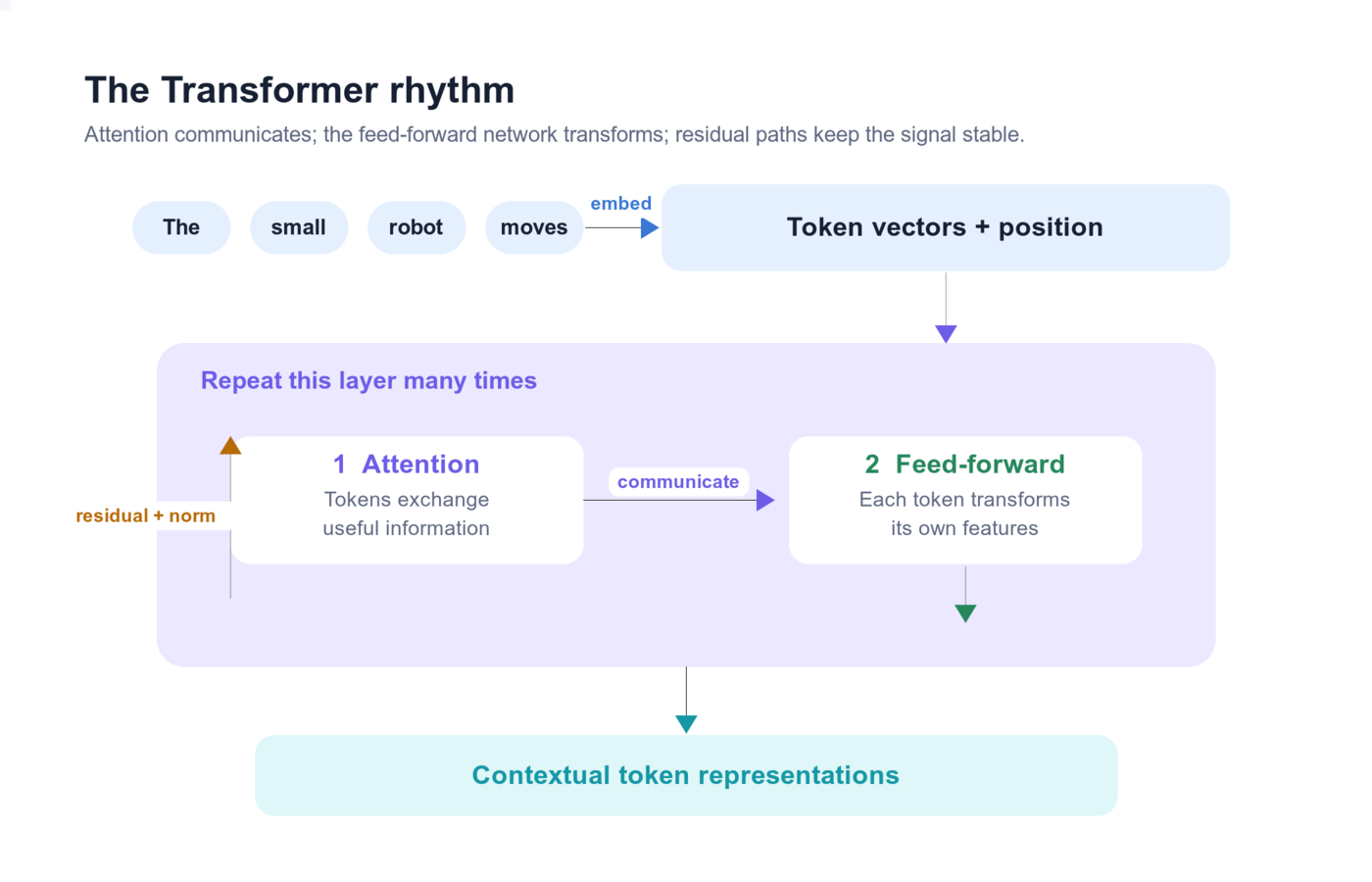
Diagram 1 — The repeating Transformer rhythm. Attention communicates across positions; the feed-forward network transforms each position.
What made this design a breakthrough?
The 2017 paper Attention Is All You Need removed recurrence from its encoder-decoder model. That brought three large advantages:
- Shorter information paths: two far-apart tokens can interact through one attention calculation instead of passing a message through every token between them.
- Parallel work over known positions: during training, the input positions can be processed together on GPUs and TPUs.
- A reusable architecture: the same core blocks can process text, image patches, audio frames, biological sequences, and other token-like inputs.
One qualification matters:
A Transformer can process the known positions of a training sequence or prompt prefill in parallel. A normal autoregressive decoder still generates new tokens one at a time, because the next token does not exist until the previous one has been chosen.
2. Before Transformers: RNNs, LSTMs, and GRUs
Recurrent neural networks: update a state in sequence
A recurrent neural network (RNN) reads a sequence in order. At step t, it combines the current input x_t with a hidden state h_(t-1) from the previous step and produces a new hidden state h_t.
h_t = f(x_t, h_(t-1))
Information from an early input influences later outputs through repeated hidden-state updates. For a five-token sequence, the path from token 1 to token 5 crosses four recurrent transitions.
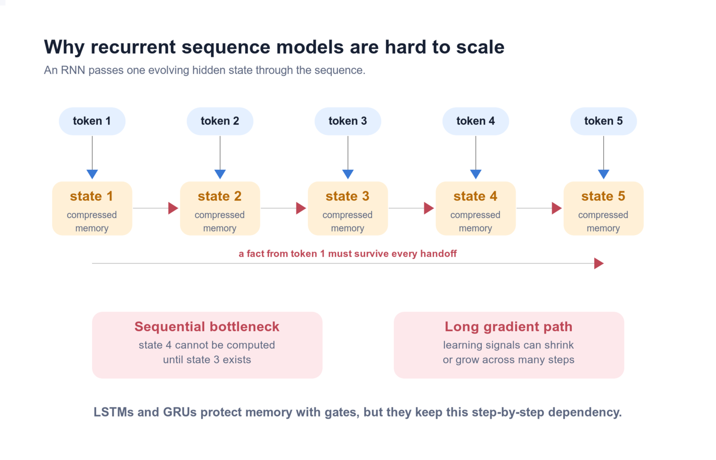
Diagram 2 — An RNN's hidden state travels through the sequence one step at a time.
This creates three problems:
- Limited parallelism: step 4 needs the state from step 3, so the steps cannot all run at once.
- Long information paths: information from the beginning must survive many updates to affect the end.
- Unstable gradients: repeated multiplication during training can make learning signals shrink toward zero or grow uncontrollably. These are called vanishing and exploding gradients.
LSTMs and GRUs: add gates to protect memory
Long Short-Term Memory networks (LSTMs) and Gated Recurrent Units (GRUs) improved recurrent models by adding learned gates. A gate is like a valve with values between 0 and 1: it controls how much information to keep, write, or reveal.
- An LSTM has a separate cell-state memory and input, forget, and output gates. Its cell update adds retained old memory to gated new information; the output gate controls the exposed hidden state.
- A GRU combines some of those ideas into a simpler update and reset-gate design.
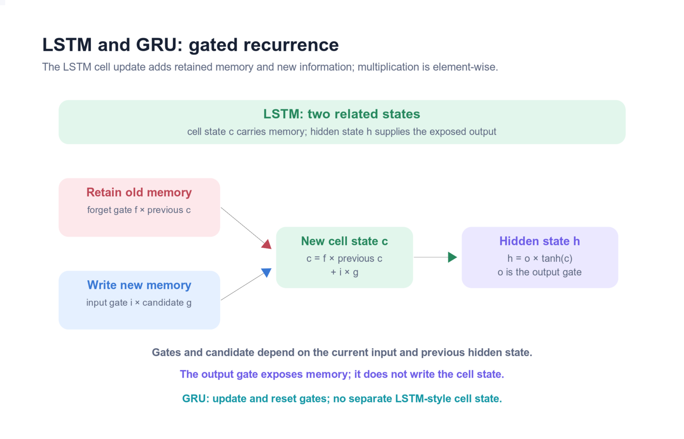
Diagram 3 — Gates help useful memories survive, but the sequence is still processed step by step.
LSTMs and GRUs made longer dependencies easier to learn, but they did not remove the sequential bottleneck. Transformers changed the route entirely: tokens communicate through attention rather than one shared state moving along a chain.
RNN family versus Transformer
| Question | RNN / LSTM / GRU | Transformer |
|---|---|---|
| How does information travel? | Through a recurrent hidden state | Directly between allowed positions through attention |
| Can known training positions run in parallel? | Mostly no | Largely yes |
| Path between distant tokens | Grows with their distance | Can be one attention step |
| Main long-sequence challenge | Sequential bottleneck and memory loss | Attention cost and finite context |
| Does generation become fully parallel? | No | No for ordinary autoregressive decoding |
3. The Original Encoder-Decoder Transformer
The original Transformer was built for sequence-to-sequence tasks such as translation. It has two stacks:
- The encoder reads the complete source sequence and builds a contextual representation at every source position.
- The decoder produces the target sequence one token at a time. It uses its earlier target tokens plus information from the encoder.
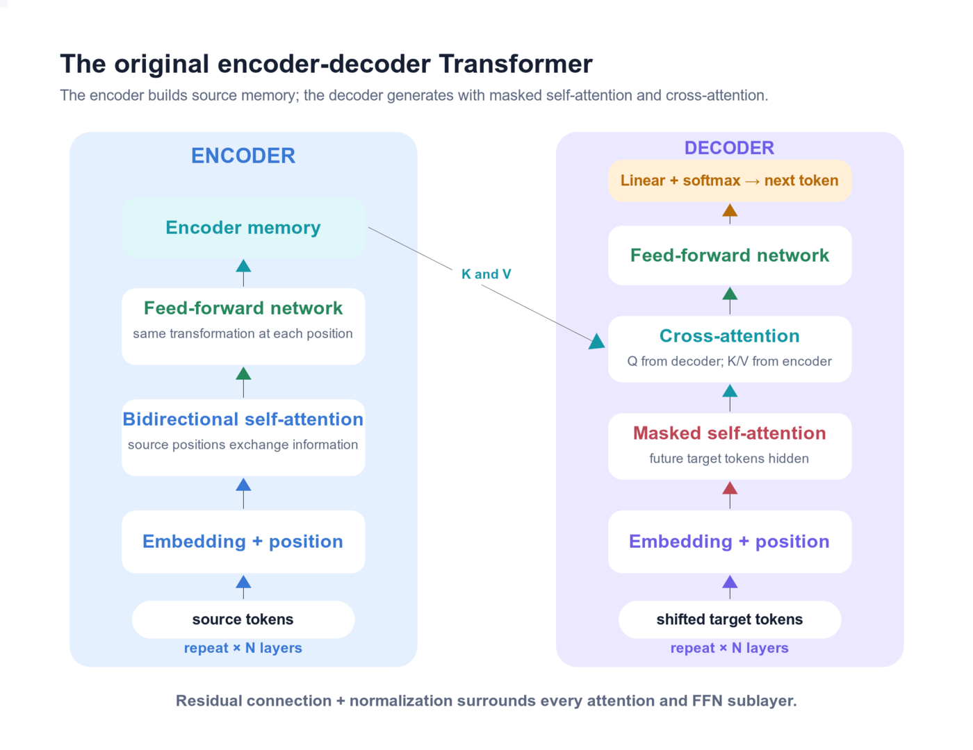
Diagram 4 — The original Transformer. “Add & Norm” means a residual addition followed by normalization in the 2017 post-norm design.
One encoder layer contains
- multi-head bidirectional self-attention,
- a position-wise feed-forward network,
- a residual connection and normalization around each sublayer.
“Bidirectional” means each source position can use tokens on both sides when the complete input is known.
One decoder layer contains
- masked multi-head self-attention over the target prefix,
- cross-attention to the encoder output,
- a position-wise feed-forward network,
- residual connections and normalization.
The decoder's mask hides future target tokens. Without it, training would let the model look at the answer it is supposed to predict.
A stack repeats the structure with separate parameters
The diagram shows one encoder layer and one decoder layer, but production models stack many layers. Each layer receives the previous layer's representations and produces refined ones. Unless an architecture deliberately shares parameters, every layer has its own learned weights.
4. Input Processing: Tokens, Embeddings, and Position
A Transformer cannot receive the sentence Birds fly south directly. The input must become numbers with useful shapes.
Step 1: tokenize the input
A tokenizer splits the input into pieces and maps each piece to an integer ID.
"Birds fly south" → ["Bird", "s", " fly", " south"] → [7312, 82, 2249, 5140]
The exact pieces and IDs depend on the tokenizer. The ID 7312 is only a lookup address; its size does not represent how “bird-like” the token is. See Tokenization Deep Dive for BPE, WordPiece, Unigram, special tokens, and multilingual trade-offs.
Step 2: look up token embeddings
The model has an embedding table with one learned vector per vocabulary item.
embedding table shape = vocabulary_size × d_model
Looking up four IDs returns four vectors:
token IDs shape  = 4
embeddings shape = 4 × d_model
An embedding is the token's starting representation. After Transformer layers mix in context, it becomes a contextual hidden state.
Step 3: add or apply position information
Unmasked self-attention without position-dependent inputs or biases is permutation-equivariant: reordering input vectors reorders the outputs in the same way. A model needs an ordering mechanism to distinguish sequence relationships such as dog bites person versus person bites dog.
Depending on the model, position can be:
- added to token embeddings, as with learned absolute or sinusoidal vectors;
- applied inside attention, as with rotary position embedding (RoPE);
- added as a distance-dependent bias to attention scores, as with ALiBi.
5. Self-Attention, Step by Step
Suppose the model reads:
The animal crossed the street because it was quiet.
In a bidirectional encoder, to build a useful representation for it, the model may need information from animal, street, and quiet. Self-attention gives the it position a learned way to collect that information.
Query, key, and value
Every token representation is projected into three new vectors for each attention head:
- Query (Q): what information is this position looking for?
- Key (K): what kind of information can this position be matched on?
- Value (V): what information should this position contribute if selected?
A library analogy helps:
- Your search request is the query.
- Each catalog label is a key.
- The book content you retrieve is the value.
Q, K, and V are runtime activations. The projection matrices W_Q, W_K, and W_V are learned parameters.
Q = XW_Q
K = XW_K
V = XW_V
Score each allowed key
For one query, dot products compare it with all allowed keys. Large positive scores mean “this key looks useful to this query.”
scores = QKᵀ
If the sequence has n positions, the score matrix is n × n: one row per query position and one column per key position.
Scale the scores
When the key/query dimension d_k grows, raw dot products tend to grow in magnitude. Very large values can push softmax into nearly flat-gradient regions. Dividing by sqrt(d_k) keeps their typical scale manageable.
scaled scores = QKᵀ / sqrt(d_k)
Apply a mask when needed
An additive mask uses zero for allowed keys and negative infinity for forbidden keys. Softmax assigns forbidden keys zero weight when the row has at least one finite allowed score. A finite approximation must be sufficiently negative for the chosen dtype; an entirely blocked row needs explicit handling rather than an undefined all-negative-infinity softmax.
Turn scores into weights
Softmax converts each row of scores into nonnegative weights that sum to 1.
weights = softmax(scaled scores + mask)
Mix the values
The weights produce a weighted sum of value vectors.
output = weights × V
The complete equation is:
Attention(Q, K, V) = softmax(QKᵀ / sqrt(d_k) + M)V
Here M is the additive mask, expressed with zero for allowed positions and negative infinity for forbidden ones. The mask is added to the scaled scores before softmax.
What self-attention buys us
- Context-aware representations: the representation of
bankcan change betweenriver bankandbank loan. - Direct long-range connections: distant positions can interact without a recurrent chain.
- Parallel computation over known positions: all queries can be evaluated with large matrix operations.
The cost
A straightforward full-attention implementation materializes an n × n score matrix per head, giving quadratic score storage and query-key work in sequence length. FlashAttention computes full attention with a different tiled execution order, avoiding storage of the whole score matrix in slow memory. It preserves the mathematical attention operation, subject to floating-point differences, but full attention still has quadratic query-key interactions. FlashAttention.
6. Multi-Head Attention
One attention operation has one learned matching space. Multi-head attention runs several smaller attention operations in parallel, concatenates their outputs, and projects the combined result back to the model width.
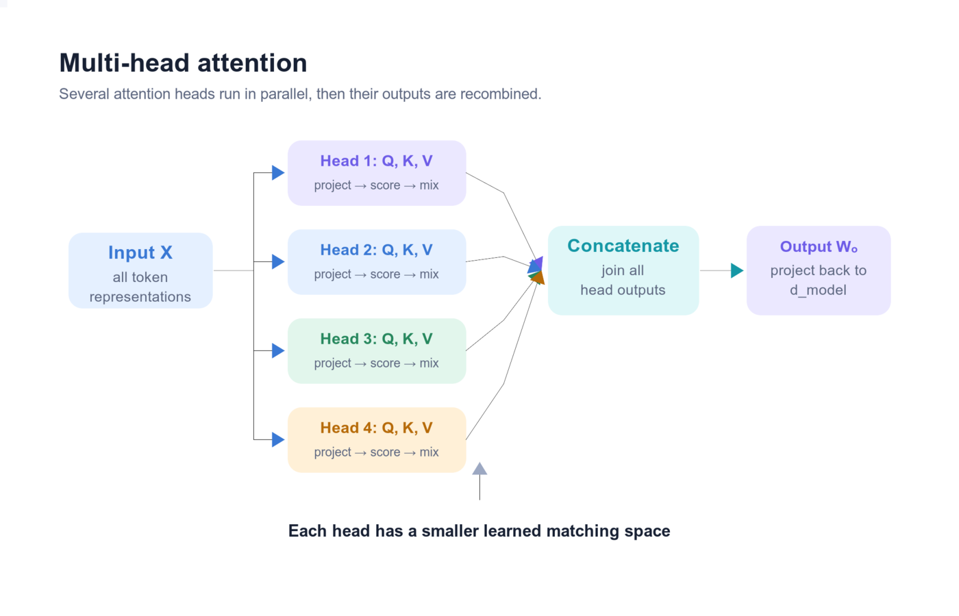
Diagram 5 — Multiple heads provide multiple learned ways to match and move information.
For h heads:
head_i = Attention(Q_i, K_i, V_i)
MultiHead(X) = Concat(head_1, ..., head_h)W_O
In a standard design:
d_head = d_model / h
Splitting into heads does not necessarily multiply the final model width. The head outputs concatenate back to d_model before the output projection.
Do heads learn different jobs?
Heads can learn different patterns: nearby syntax, delimiter structure, repeated names, pronoun links, or task-specific relationships. This gives the layer several representation subspaces at once.
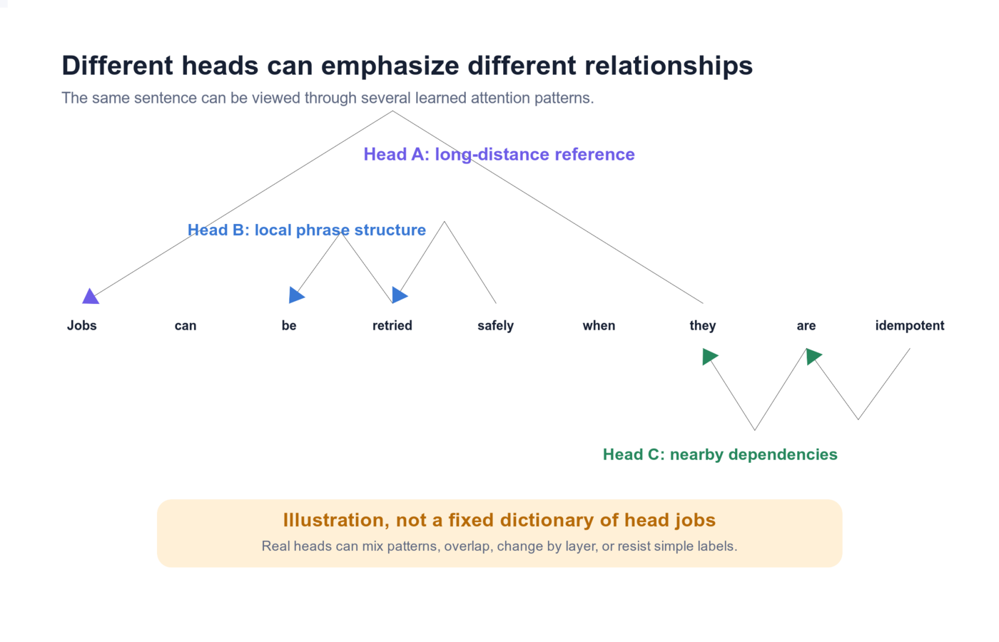
Diagram 6 — Illustrative attention patterns. Real learned heads may be mixed, redundant, difficult to name, or prunable.
Do not turn this intuition into a rigid claim that “head 3 always tracks pronouns.” Researchers sometimes find interpretable patterns, but a head's behavior can vary by layer, input, and model.
MHA, MQA, and GQA
Modern decoders often reduce the number of key/value heads to shrink the K/V cache:
| Design | Query heads | Key/value heads | Main trade-off |
|---|---|---|---|
| MHA | many | one per query head | Most independent K/V projections; largest cache |
| MQA | many | one shared K/V head | Smallest cache; more sharing |
| GQA | many | several shared K/V groups | Middle ground between MHA and MQA |
The attention idea stays the same; the sharing pattern changes.
7. Positional Information
Unmasked attention alone does not encode sequence order. Explicit position signals make ordering and distance available to the network. A causal mask also breaks permutation symmetry by changing which prefixes each position can see; some causal models learn positional behavior without explicit positional embeddings. Do not extend the unmasked result into a claim that every causal model must have a position table or RoPE. Position-encoding study.
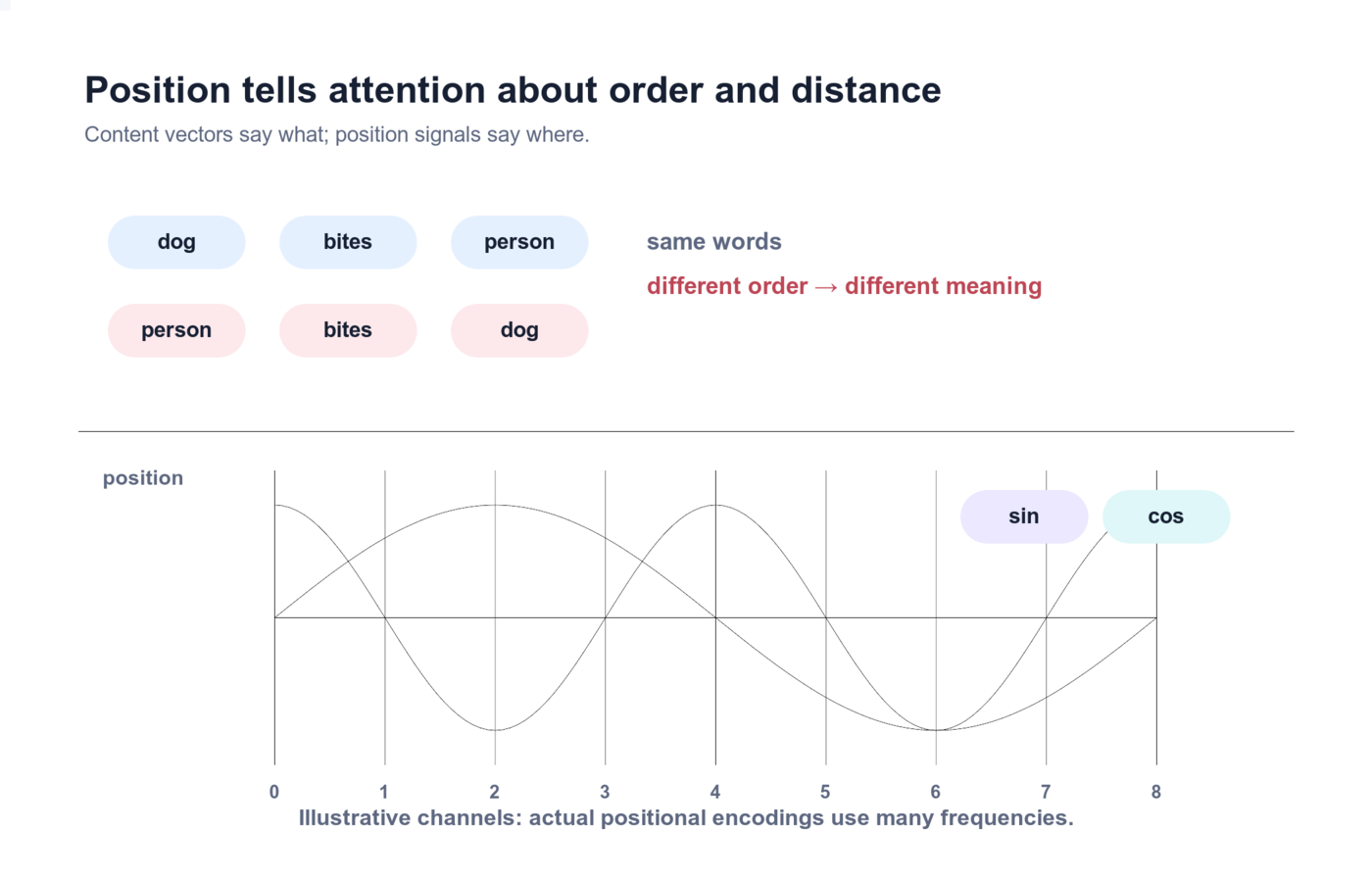
Diagram 7 — Content says what a token is; position says where it is.
Original sinusoidal encoding
The 2017 Transformer added sine and cosine waves of different frequencies to token embeddings:
PE(pos, 2i)     = sin(pos / 10000^(2i / d_model))
PE(pos, 2i + 1) = cos(pos / 10000^(2i / d_model))
You do not need to memorize the formula first. The intuition is that every position receives a distinctive combination of slow and fast waves, like several clock hands turning at different speeds.
Why use sinusoids?
- They require no learned table.
- Their smooth structure exposes relative offsets through predictable relationships.
- They can be evaluated at positions beyond those stored in a fixed learned table, although useful long-length generalization is not guaranteed merely by evaluating the formula farther out.
Learned absolute positions
The model can instead learn one position vector for position 0, another for position 1, and so on. This is simple, but the table has a designed maximum length and does not itself explain how to extend beyond training positions.
RoPE and relative methods
Many modern language models use RoPE, which rotates pairs of Q and K features by position-dependent angles. The resulting dot products naturally contain relative-position information. Other models use learned relative biases or ALiBi-style distance biases.
Position is not a single solved component: the choice affects long-context behavior, extrapolation, and attention efficiency.
8. Feed-Forward Networks
Attention communicates between positions. The feed-forward network, or FFN, transforms each position independently using the same learned function.
The FFN receives already-contextual representations. “Independently” means it does not directly read other positions during that sublayer, not that its inputs contain no context.
The original Transformer used a two-layer multilayer perceptron:
FFN(x) = ReLU(xW_1 + b_1)W_2 + b_2
It usually:
- expands from
d_modelto a widerd_ff, - applies a nonlinear activation,
- contracts back to
d_model.
The same FFN weights are applied at every sequence position, but each position has different activations. Returning to d_model is important because the output must be added to the residual stream.
Modern models may replace ReLU with GELU, SiLU, or a gated form such as SwiGLU. Some replace the one dense FFN with a mixture of experts (MoE) router that sends each token to a small subset of several FFN experts.
9. Residual Connections and Normalization
A deep model needs a reliable route for information and gradients. Transformer layers use residual connections:
output = input + sublayer_update
Instead of asking each sublayer to rebuild the whole representation, it only needs to propose an update.
Layer normalization then controls the scale of a token's features. For one token vector, LayerNorm subtracts that vector's feature mean, divides by its feature standard deviation, then applies learned scale and shift parameters in the standard affine form. An epsilon inside the square root prevents division by zero.
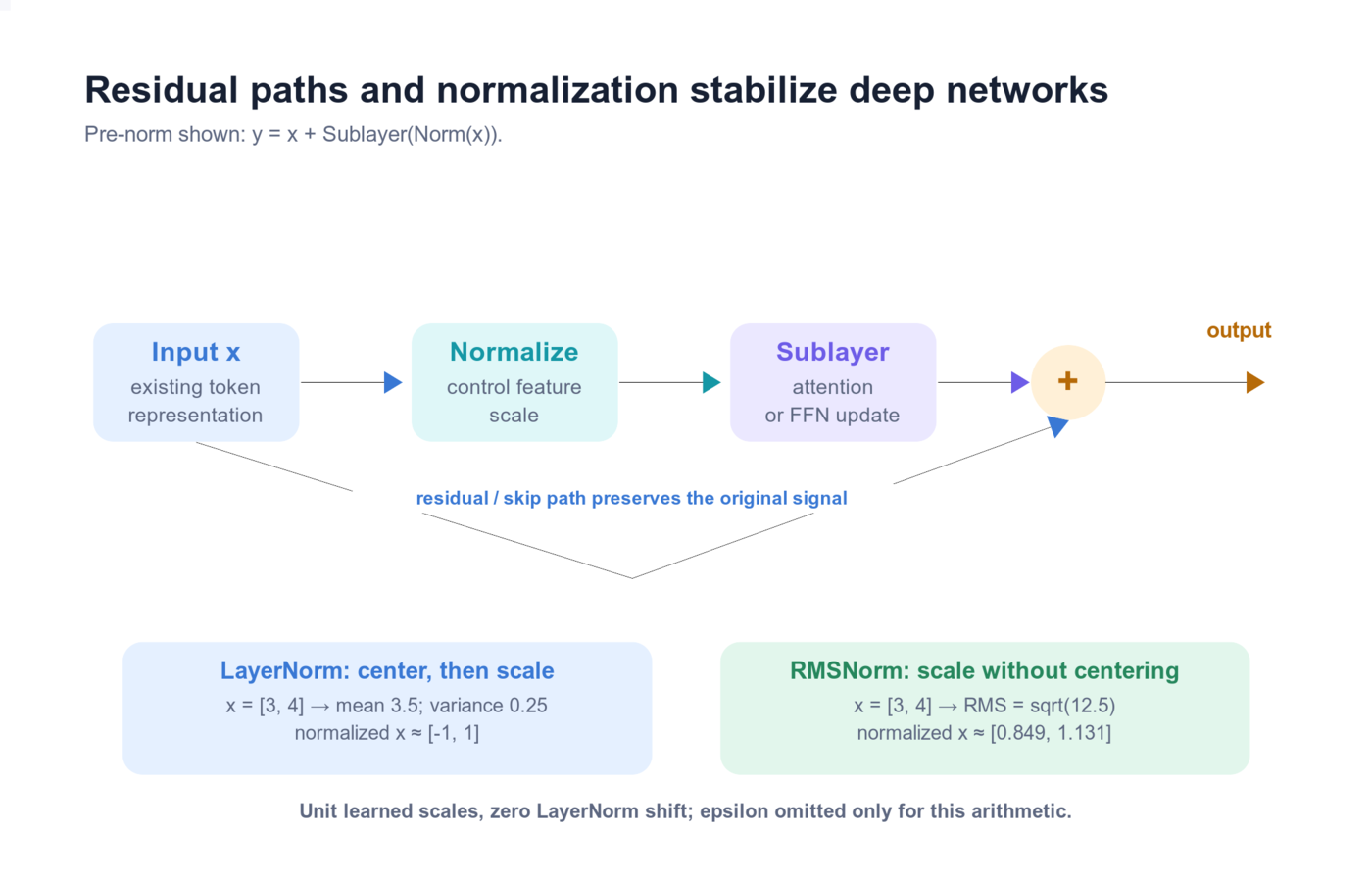
Diagram 8 — Residual paths preserve information; normalization makes optimization more stable.
LayerNorm normally normalizes across the feature dimension of each token, not across all tokens in the sequence. It does not make all token representations the same.
Post-norm versus pre-norm
The original Transformer used post-norm:
y = LayerNorm(x + Sublayer(x))
Many modern deep Transformers use pre-norm:
y = x + Sublayer(Norm(x))
Pre-norm gives gradients a more direct residual path and often improves optimization stability. It does not guarantee better final quality, remove all gradient problems, or universally eliminate learning-rate warmup. Modern language models also often use RMSNorm, which scales by root-mean-square magnitude without subtracting the mean. Normalization placement and normalization formula are separate choices. Pre-norm analysis, RMSNorm.
Work through the modern FFN and normalization formulas
For a bias-free SwiGLU FFN, let the model width be d and the intermediate width be f:
up   = x W_up          W_up:   d × f
gate = SiLU(x W_gate)  W_gate: d × f
out  = (gate ⊙ up) W_down      W_down: f × d
SiLU(z) = z × sigmoid(z)
Here ⊙ means element-wise multiplication. The gate is SiLU-transformed; unlike an LSTM's sigmoid gate, its values are not limited to 0–1. There are three projection matrices, so the main parameter count is 3df. A two-matrix FFN with width 4d has 8d² weights. Matching that budget gives a SwiGLU width near 8d/3, often rounded for hardware efficiency. It is not a required expansion factor for every model. GLU variants.
| Normalization | Formula for one token's feature vector | What changes? |
|---|---|---|
| LayerNorm | γ ⊙ (x − mean(x)) / sqrt(variance(x) + ε) + β |
Centers and rescales features, then applies learned affine parameters |
| RMSNorm | γ ⊙ x / sqrt(mean(x²) + ε) |
Rescales without subtracting the mean; commonly has learned scale only |
For x = [3, 4], unit learned scales, zero shift and epsilon omitted only for arithmetic:
- LayerNorm has mean 3.5 and variance 0.25, producing
[-1, 1]. - RMSNorm has RMS
sqrt(12.5) ≈ 3.536, producing[0.849, 1.131].
These operations do not guarantee that every coordinate shrinks or that representations become equal. Learned scale and shift parameters also change the result. Actual implementations keep epsilon and choose stable accumulation precision.
10. Causal Masking
An autoregressive decoder predicts a token using only the prefix available before that prediction. During training, the complete target sentence is already present, so a mask must enforce that rule.
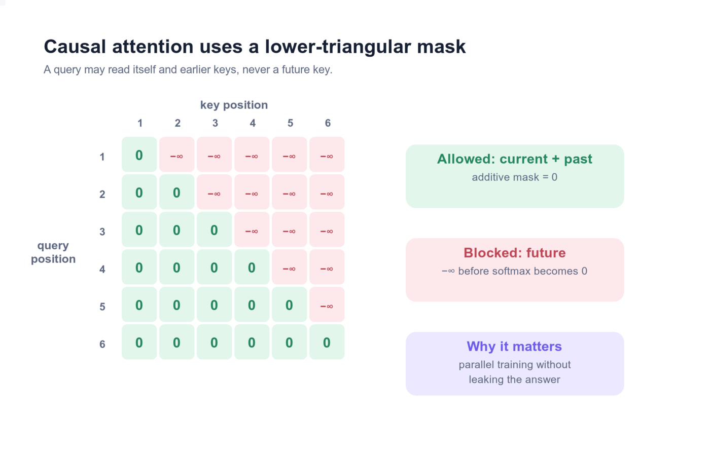
Diagram 9 — Query row t may attend only to key columns ≤ t.
For four positions, the allowed pattern is:
          keys
          1  2  3  4
query 1   ✓  ·  ·  ·
query 2   ✓  ✓  ·  ·
query 3   ✓  ✓  ✓  ·
query 4   ✓  ✓  ✓  ✓
Forbidden logits receive -∞ (or a sufficiently negative finite value) before softmax:
softmax([2.1, 0.7, -∞, -∞]) → [0.80, 0.20, 0.00, 0.00]
Align input positions with prediction targets
A decoder input such as [BOS, The, cat] predicts [The, cat, sleeps]. The state at cat may read cat and earlier input tokens because its target is the next token, sleeps. The mask and this one-position shift work together; feeding each target at its own prediction position leaks the label. Padding positions also need exclusion from attention and from the training loss as appropriate.
Why training can still be parallel
The correct earlier tokens come from the training example, so the model can compute predictions at every position together. The triangular mask prevents information leakage while matrix operations remain parallel.
During generation, the true future tokens are unknown. The decoder must select a token, append it, and run the next decode step. The K/V cache avoids recomputing keys and values for the old prefix, but it does not make future token choices exist in advance.
11. Cross-Attention
Self-attention uses Q, K, and V from the same sequence. Cross-attention connects two sequences:
- Queries come from the decoder's current hidden states.
- Keys and values come from the encoder's final representations.
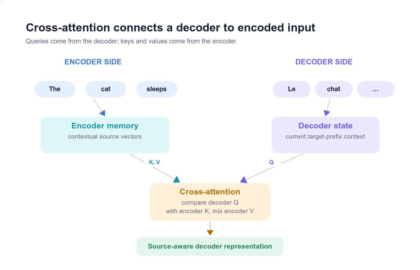
Diagram 10 — The decoder asks the encoded source, “Which source information helps me write the next target token?”
Imagine translating The cat sleeps into French. When producing chat, a decoder query can place a large weight on the encoder representation for cat. It is not copying a dictionary entry; it is retrieving a learned mixture of contextual source information.
Cross-attention supports tasks where outputs must stay connected to a separate input:
- translation,
- abstractive summarization,
- question answering over an encoded passage,
- image captioning when text decoding attends to visual tokens,
- speech recognition when text decoding attends to audio representations.
A complete encoder-decoder layer flow
source tokens
  → encoder self-attention
  → encoder FFN
  → source memory (K and V for decoder cross-attention)

target prefix
  → masked decoder self-attention
  → cross-attention using decoder Q and encoder K/V
  → decoder FFN
  → next-target-token logits
This is a useful engineering description. “The encoder understands and the decoder writes” is a memorable shortcut, but both sides are learned numerical transformations rather than separate human-like faculties.
12. Encoder-Only, Decoder-Only, and Encoder-Decoder Families
The word Transformer names a toolkit, not one fixed product.
| Family | Attention visibility | Common training objective | Good fit | Classic example |
|---|---|---|---|---|
| Encoder-only | Both left and right within the input | Reconstruct masked/corrupted input | Classification, tagging, retrieval embeddings | BERT |
| Decoder-only | Current and earlier input positions; predict the next token | Predict the next token | Open-ended generation and chat | GPT-style models |
| Encoder-decoder | Encoder sees complete source; decoder sees target prefix and encoder memory | Generate a target from a source | Translation, summarization, structured transformation | T5 |
Encoder-only: build representations from complete input
BERT-style models use bidirectional attention because the whole input is available. They are strong when the output is a label or representation rather than a long generated continuation.
Decoder-only: repeatedly predict the next token
GPT-style models use causal attention. A chat prompt, tool result, document, and earlier generated answer can all be placed in one token sequence. The model repeatedly produces next-token logits.
Encoder-decoder: separate source reading from target writing
T5-style models are natural when there is a clear input sequence and output sequence. The encoder can process the source once, and the decoder can cross-attend to that source while generating.
Architecture family, training objective, and product behavior are different labels. “Chat model,” “reasoning model,” or “multimodal model” does not by itself prove which internal family is used.
13. Scaling Transformers
Scaling means increasing the resources that let a model learn a more capable function. Four dimensions must be considered together.
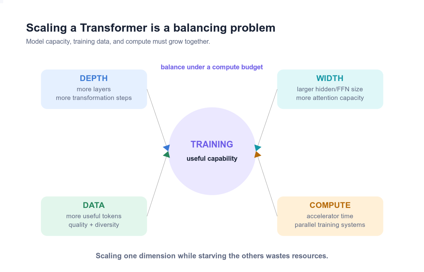
Diagram 11 — Bigger models help only when data, compute, optimization, and evaluation keep pace.
Depth
Add more Transformer layers. Greater depth lets representations pass through more rounds of communication and transformation, but it increases training difficulty, latency, and memory use.
Width
Increase d_model, head count or head dimension, and FFN size. Wider layers can represent and transform more features, but matrix multiplications become more expensive.
Data
Train on more tokens and broader, higher-quality distributions. Repeating low-quality or narrow data is not equivalent to adding useful data. Deduplication, mixture design, contamination controls, and curriculum all matter.
Compute
Use more accelerator time for forward passes, backward passes, and optimizer updates. Large training runs combine techniques such as:
- mixed precision (for example BF16 activations with carefully chosen accumulation precision),
- data parallelism,
- tensor parallelism,
- pipeline parallelism,
- expert parallelism for MoE models,
- activation checkpointing and optimizer-state sharding.
Compute-optimal balance
Empirical scaling laws show that model size and training-token count should grow together under a fixed training-compute budget. A model that is enormous but trained on too little data can be undertrained; a tiny model trained on far more data eventually becomes capacity-limited.
The often-quoted Chinchilla-era rule of roughly 20 training tokens per parameter was an estimate under particular model, data, and compute assumptions—not a universal physical law. Teams may train smaller models on more tokens than that compute-optimal training point when the extra one-time training cost reduces repeated inference cost.
How the main families scale
- BERT-style encoders scale bidirectional representation learning, often with masked-token objectives.
- GPT-style decoders scale causal next-token prediction and generation.
- T5-style encoder-decoders scale source-to-target text transformation.
All three can grow in depth, width, data, and compute. Their attention patterns and training objectives make their serving behavior different.
14. Important Transformer Variants
The core pattern—attention, per-position transformations, residual paths, normalization, and position information—has been adapted in many ways.
BERT
BERT is an encoder-only Transformer pretrained to reconstruct masked tokens (with an additional next-sentence prediction objective in the original recipe). Because its attention sees both sides of a token, it became a foundation for language understanding, tagging, classification, and embeddings.
ALBERT
ALBERT reduces parameter count mainly through:
- factorizing the large vocabulary embedding parameters from the hidden width,
- sharing parameters across layers.
It can therefore build a deep network without giving every layer a completely separate copy of all parameters. Sharing reduces stored parameters; it does not make the repeated layer computations disappear.
XLNet
XLNet uses a permutation language-modeling objective. Instead of replacing input tokens with mask tokens, it trains across different factorization orders so a representation can learn from context on both sides while retaining an autoregressive objective. It also incorporates ideas from Transformer-XL for longer context.
“Permutation” describes the order used for the prediction objective, not randomly scrambling the sentence presented to the model.
RoBERTa
RoBERTa kept BERT's basic encoder architecture and showed how much the training recipe mattered. It trained longer on more data with larger batches, removed next-sentence prediction, used longer sequences, and changed masks dynamically.
Its lesson is broader than one model: an apparent architecture improvement can sometimes be a data or optimization improvement.
DistilBERT
DistilBERT compresses a BERT teacher into a smaller student through knowledge distillation. The student learns both from the original language-modeling task and from signals produced by the larger teacher.
The goal is a better speed-memory-quality trade-off, not a new attention mechanism.
Vision Transformer (ViT)
ViT divides an image into fixed-size patches, flattens and projects each patch into a vector, adds position information, and sends the patch sequence through a Transformer encoder.
image → grid of patches → patch vectors → Transformer → image representation
An image patch plays a role similar to a text token. ViT showed that, with enough data and compute, a pure Transformer can be highly effective for vision without a convolutional backbone.
Modern efficiency variants
Modern models also change components inside the block:
- RoPE or relative-position methods instead of fixed absolute positions,
- RMSNorm and pre-norm layouts for stable deep training,
- SwiGLU or other gated FFNs,
- GQA/MQA to reduce K/V-cache memory,
- FlashAttention kernels to reduce attention memory traffic,
- sliding-window or sparse attention to limit long-context work,
- MoE layers to increase total capacity while activating only some experts per token,
- Multi-head Latent Attention (MLA) to compress attention state in documented architectures that use it.
These variants keep enough of the original pattern to remain recognizably Transformer-based, but they solve different bottlenecks and should not be treated as synonyms.
Read current model configurations instead of guessing internals
Architecture observations checked on 24 September 2026:
| Documented example | What the source establishes | System implication |
|---|---|---|
| DeepSeek-V3 | 61 Transformer layers in its configuration; MLA attention and routed/shared experts in the technical report | Plan latent attention state and expert communication; neither ordinary MHA cache sizing nor active-parameter count alone gives total serving memory |
| Qwen3.8-27B | Its text configuration has 64 layers, with three linear-attention layers followed by one full-attention layer; width 5,120, full-attention head dimension 256 and 24 query heads | A hybrid has different state types. Also, query-head count × head width need not equal the residual-stream width |
| Closed model APIs | Public capability and limit documentation may omit layer count, position method, expert routing and weight tying | Treat undisclosed internals as unknown; size the application from measured behavior and documented limits |
Sources: DeepSeek-V3 configuration, technical report, Qwen configuration. These are architecture examples, not a ranking or a recommendation to choose a model solely because it is newer.
Mixture of experts: a router selects a subset of FFN experts for a token and combines their outputs. Total parameters describe stored capacity; active parameters describe the subset used in a forward path. Unselected experts still need storage or an explicit offload mechanism. Expert parallelism can add all-to-all transfers, uneven expert loads and queueing. Shared experts and dense layers are model-specific choices, not a universal schedule that guarantees “global knowledge.”
Hybrid sequence models: some layers use a recurrent or linear-attention state while others use full attention. This changes memory growth and retrieval behavior. It does not make full-attention layers free or justify applying the same KV-cache formula to every layer.
Sliding windows: limiting each layer to a local window can reduce attention work and retained state. Information may travel farther through stacked layers, but this is not equivalent to every layer directly attending to the whole document. The actual trained context limit, attention pattern and long-range task quality still matter.
MLA: multi-head latent attention uses compressed attention state in architectures designed for it. It is different from simply quantizing an ordinary cache, and it does not compress every other part of the model. See attention mechanisms for the representations and implementation tradeoffs.
15. Applications Beyond Chat
Transformers can be applied to many problems represented as input units with relationships between them. Suitability still depends on data, objective and computational budget.
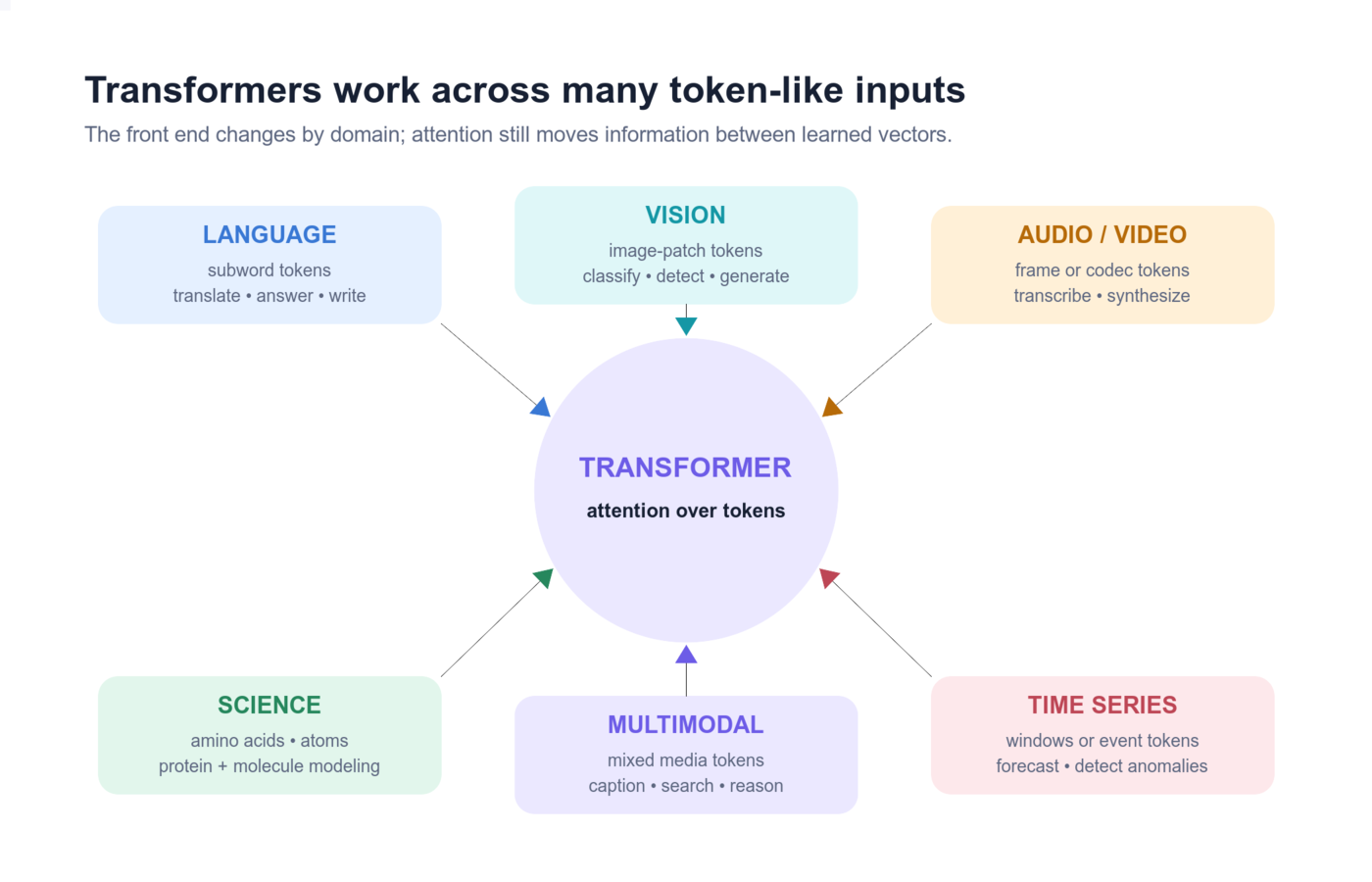
Diagram 12 — The input units change by domain; the attention-based information exchange remains recognizable.
| Domain | What acts like a token? | Example outputs |
|---|---|---|
| Natural language | Subword or byte pieces | Translation, summarization, search, question answering, chat |
| Vision | Image patches or learned visual tokens | Classification, detection, segmentation, image generation |
| Audio and speech | Time-frequency patches, codec tokens, or learned frames | Transcription, synthesis, music modeling |
| Multimodal systems | Interleaved text, image, audio, or video tokens | Visual question answering, captioning, media generation |
| Biology and chemistry | Amino acids, nucleotides, atoms, or learned structural units | Protein modeling, molecular property prediction, drug discovery support |
| Time series | Time windows, measurements, or event tokens | Forecasting, anomaly detection, event prediction |
A shared architecture does not mean identical preprocessing. A tokenizer for text, a patch projector for images, and an audio codec solve different input problems before the Transformer sees vectors.
16. A Complete Forward Pass
Follow a decoder-only model generating one token after the prompt:
The small robot picked up the
1. Tokenize
The text becomes token IDs. The model also receives any system, user, or tool-message control tokens defined by its chat template.
2. Embed and add position information
Each token ID selects a vector from the embedding table. The model adds or applies a position mechanism.
3. Enter a Transformer layer
For a modern pre-norm layer:
h = x + Attention(Norm(x))
y = h + FFN(Norm(h))
4. Build Q, K, and V
Learned projections turn normalized hidden states into queries, keys, and values. A positional operation such as RoPE may transform Q and K.
5. Apply causal self-attention
Each prompt position can gather information only from itself and earlier positions. During prefill, all prompt positions are computed together under that mask.
6. Run the FFN
Every position independently passes through the same FFN parameters. The residual path adds the update back to the stream.
7. Repeat through all layers
Later layers work with increasingly contextual hidden states.
8. Produce logits
The final hidden state at the last prompt position is normalized and projected to one raw score per vocabulary token.
last hidden state: 1 × d_model
vocabulary matrix: d_model × vocabulary_size
logits:             1 × vocabulary_size
9. Select the next token
Softmax and a decoding rule such as greedy choice, temperature plus top-p, or another sampler choose a token such as box.
10. Decode again
The model appends box, processes the new position, extends each layer's K/V cache, and predicts the following token. Learned model weights remain fixed during normal inference.
17. Common Misunderstandings
“Transformers process everything in parallel”
They parallelize work across already-known positions during training and prompt prefill. Standard autoregressive generation still depends on earlier generated tokens.
“Attention is the entire Transformer”
Attention moves information between positions. FFNs, residual paths, normalization, embeddings, position mechanisms, and the output head are also essential.
“A high attention weight is a complete explanation”
An attention matrix shows one internal routing pattern. Residual mixing, other heads, FFNs, and later layers also shape the result. Attention can be useful evidence without being a complete causal explanation.
“Each attention head has one English name”
Some heads show interpretable patterns, but roles can overlap, change by input, or resist simple labels.
“The decoder is the only generative component”
In an encoder-decoder model, the decoder emits target tokens. A decoder-only model is also generative even though it has no separate encoder stack.
“Position encoding is always added to embeddings”
That is true for the original sinusoidal scheme and learned absolute embeddings. RoPE changes Q and K inside attention; ALiBi adds a bias to attention scores.
“Larger always means better”
Capability depends on the balance of architecture, data, compute, objective, optimization, and evaluation. More parameters alone do not guarantee a better or safer model.
Worked parameter count: build the total from the parts
Assume a hypothetical dense decoder with vocabulary V = 32,000, width d = 4,096, L = 32 layers, ordinary multi-head attention, and gated FFN width f = 11,008. Ignore small norm parameters and biases initially. These are arithmetic assumptions, not a named model's complete configuration.
| Component | Why this many weights? | Count |
|---|---|---|
| Token embedding | One width-4,096 vector for each vocabulary item: Vd |
131,072,000 |
| Attention in one layer | Q, K, V, and output projections: 4d² |
67,108,864 |
| Gated FFN in one layer | Gate and up projections d × f, plus down projection f × d: 3df |
135,266,304 |
| All 32 blocks | 32 × (67,108,864 + 135,266,304) |
6,476,005,376 |
| Untied output head | A separate hidden-to-vocabulary matrix: dV |
131,072,000 |
| Total, untied | Embedding + blocks + separate output head | 6,738,149,376 |
| Total, tied | Reuse embedding weights for the output head | 6,607,077,376 |
Weight tying saves 131,072,000 stored parameters in this example. It does not remove the final vocabulary projection computation. At two bytes/weight, ideal untied storage is 13.48 decimal GB, versus 13.21 GB tied. Add norm parameters, buffers, cache, workspace, and allocation overhead before claiming it fits on a device. Training adds gradients, optimizer state, saved activations, and possibly master weights; do not reuse the inference-only total.
GQA changes the count: if 32 query heads share eight KV heads at width 128, Q and output remain d × d, while K and V each become d × 1024. Attention parameters fall from 67,108,864 to 41,943,040 per layer. The FFN and vocabulary matrices do not shrink just because KV heads shrink.
A matrix-vector multiply uses approximately two floating-point operations per weight under the usual multiply-plus-add convention. Thus 2 × parameters is a useful rough dense linear-layer estimate per generated token, but attention over cached positions adds work, and batching changes hardware efficiency. For the derivation of storage, follow weight memory versus parameter count and the KV-cache formula.
For an MHA block with a two-matrix FFN of width 4d, attention contributes 4d² and the FFN 8d², giving the familiar 12Ld² block estimate. A three-matrix SwiGLU FFN of width 4d instead gives 16Ld². Vocabulary matrices and smaller terms must still be added. The training shorthand 6 × parameters × training tokens assumes a dense regime where parameter-matrix operations dominate; long-sequence attention, MoE routing and actual hardware efficiency need separate accounting.
Interview follow-up: Which choice saves weight memory without removing vocabulary projection work? Weight tying. Which choice mainly shrinks K/V projections and cache? GQA. These solve different costs.
Architecture selection interview: a private writing assistant
Prompt: Choose and serve a model for a private assistant that rewrites a supplied draft into a structured response. Explain the architecture, identify the first design's failures and justify a revised design.
This exercise uses hypothetical trained candidates and measured-throughput assumptions. Changing a checkpoint from MHA to GQA or changing its FFN is not a serving configuration toggle; it requires compatible trained weights and quality validation.
Functional requirements
- Accept authenticated text requests and produce a rewrite in the requested structure.
- Support up to 8,192 retained input-plus-output positions per active request, with an explicit output budget.
- Stream output, allow cancellation and report failure clearly.
- Keep each tenant's request and cached state within its authorized scope.
- Record model/release identity, usage and evaluation outcomes without logging private text by default.
Non-functional requirements
- Quality: preserve facts and requested constraints on a held-out rewrite set; measure failures separately from format validity.
- Latency: assume p95 first text below one second and a separately agreed output-token rate at peak load.
- Capacity: assume 40,000 requests/day over eight active hours, with a peak six times the active-period average.
- Memory: use 24 GiB devices; reserve 4 GiB for measured workspace and 2 GiB for headroom in the planning example.
- Recovery: tolerate one replica's loss and deploy only evaluated, versioned model/runtime combinations.
- Privacy: reject unauthorized cross-tenant cache reuse; delete transient request state according to the service's retention policy.
Start with a baseline
An encoder-decoder can separately encode a source and generate its transformation. A decoder-only instruction model can place the task and draft in one causal sequence. Evaluate both if suitable trained candidates exist. A plain encoder-only classifier does not itself provide the required autoregressive rewrite, although encoders can support routing and validation.
Start with one quality-qualified decoder replica, a request queue and a tokenizer length check. Trace the complete forward pass before optimizing. Then inspect failures:
| Baseline flaw | Repair | Cost or limitation |
|---|---|---|
| Device sizing counts only weights | Budget KV state, workspace and concurrent requests | Smaller admitted batches or additional devices |
| Long requests monopolize the queue | Bound input/output, use admission control and fair scheduling | Some requests wait or receive a clear capacity response |
| One replica fails | Multiple replicas plus one-replica spare capacity | Paid idle headroom |
| An unsupported cache-sharing optimization leaks state | Scope cache reuse by trusted tenant/group and exact model/input identity | Lower cache-hit rate |
| A faster candidate changes rewrite facts | Holdout evaluation, canary release and rollback | Review time; performance gains may be rejected |
| Client retries append duplicated output | Give a request an ID and define resume/restart behavior | State management; an interrupted stream cannot be treated as a fresh continuation blindly |
Detailed serving design
Read diagram source
flowchart LR
    C[Authenticated client] --> G[Gateway<br/>tenant scope and request ID]
    G --> T[Tokenizer and limits<br/>input plus output budget]
    T --> Q[Bounded fair queue<br/>deadline and cancellation]
    Q --> R[Pin evaluated model release<br/>route to healthy replica]
    R --> A[Replica A<br/>weights and scoped runtime state]
    R --> B[Replica B through N<br/>reserved failure capacity]
    A --> S[Stream protocol<br/>usage and completion state]
    B --> S
    S --> C
    E[Held-out rewrite evaluation<br/>load tests and memory profile] --> V[Versioned release gate<br/>canary and rollback]
    V --> R
    S --> M[Private-safe metrics<br/>quality samples by policy]
The gateway owns identity and request accounting. The serving engine owns tensor computation and KV allocation. The release record pins weights, tokenizer/template, precision, context settings and runtime version. A cancellation releases scheduling capacity only once running work has actually stopped; a disconnected client does not prove the GPU stopped computing.
Calculate memory, then measure throughput
Use the worked parameter-count example above. For the GQA candidate with 32 layers, 32 query heads, eight KV heads and head width 128, the main untied parameter count is:
Embedding plus output: 2 × 32,000 × 4,096 = 262,144,000
32 blocks: 32 × (41,943,040 attention + 135,266,304 FFN)
Total: 5,932,843,008 parameters
BF16 weight bytes: 11,865,686,016 ≈ 11.05 GiB
The ordinary GQA KV-cache formula is:
2 × layers × retained positions × KV heads × head width × bytes/element
= 2 × 32 × 8,192 × 8 × 128 × 2
= 1,073,741,824 bytes = 1 GiB per fully reserved request
The planning budget leaves 24 − 11.05 − 4 − 2 ≈ 6.95 GiB for cache: at most six fully reserved requests per device under these assumptions. This is a memory bound, not proof that six requests meet the latency target. Small parameters, allocator fragmentation and actual kernels must fit the reservations. A shorter request consumes less live KV state, but admission must also account for its allowed growth.
For the MHA variant, 32 KV heads produce four times that cache per request. GQA reduces that part by four, not the whole system by four. FlashAttention can reduce attention workspace and traffic but does not remove the persistent KV state used by ordinary autoregressive decoding.
Assume a load test of the quality-qualified candidate sustains two completed requests/second per replica at the required latency for the measured length mix. Plan at 70% of that measured rate:
Average during active hours = 40,000 / (8 × 3,600) ≈ 1.389 requests/second
Peak = 1.389 × 6 ≈ 8.333 requests/second
Planned capacity per replica = 2 × 0.70 = 1.4 requests/second
Required active replicas = ceiling(8.333 / 1.4) = 6
With one spare = 7 replicas
At a measured mean service time of two seconds, peak mean in-flight work is about 8.333 × 2 = 16.67 requests across the fleet. Tail lengths and arrival bursts still require bounded queues and per-replica memory admission. Longer outputs can invalidate both the throughput and cache assumptions.
Compare full costs and close
Illustrative monthly operating budget, with seven replicas kept warm continuously:
| Cost | Assumption | Monthly total |
|---|---|---|
| Accelerator replicas | 7 × 720 hours × $1.20/hour | $6,048 |
| Gateway, queue, metrics and network | Explicit combined estimate | $500 |
| Operations | 20 hours × $75/hour | $1,500 |
| Quality review | 4 hours × $60/hour | $240 |
| Total | 1.2 million attempts/month | $8,288 |
That is about $6.91 per 1,000 attempts. At an assumed 95% useful-completion rate, it is $7.27 per 1,000 useful completions. Rates are planning assumptions; add any training/adaptation cost when comparing candidates that require it.
Keeping replicas warm all day buys readiness but may waste money outside the eight active hours. Scheduled downscaling can save compute after measuring model load time, traffic outside the normal window and recovery behavior. A hosted candidate may cost less; compare its actual input/output billing, privacy contract and complete quality results rather than extrapolating from parameter count.
Closing answer: “I would choose a trained model family based on the rewrite task and evaluation, then derive weights and runtime-state requirements from its actual architecture. GQA addresses KV capacity; efficient attention kernels address execution cost; neither guarantees output quality. The example needs six active replicas plus one spare under measured assumptions. I would confirm the memory and latency bounds with realistic lengths, deploy a versioned canary, and compare full cost per useful completion before committing to the fleet.”
18. Understanding Checks
1. Why did Transformers train more efficiently than recurrent models on GPUs?
RNN steps depend on previous hidden states. Transformer training can compute attention and FFN operations for all known sequence positions with large parallel matrix operations.
2. Why does attention divide by sqrt(d_k)?
Larger query/key dimensions tend to produce larger dot-product magnitudes. Scaling keeps logits in a range where softmax and gradients behave more usefully.
3. Why do models use position information?
Unmasked attention without position signals is permutation-equivariant. Explicit positional methods encode ordering or distance; a causal mask itself also supplies asymmetric prefix visibility. State which setting you mean instead of claiming that all Transformers require the same positional method.
4. What does multi-head attention add?
It gives the layer several learned matching and value-mixing subspaces, then combines their results.
5. Why does a causal decoder mask future tokens during training?
The full target sequence is physically present in the batch. The mask prevents a position from reading the future token it is meant to predict.
6. Where do cross-attention's Q, K, and V come from?
Q comes from decoder hidden states. K and V come from encoder outputs.
7. What does the FFN do that attention does not?
Attention mixes information across positions. The FFN applies a nonlinear transformation independently to each position.
8. Why use residual connections?
They preserve a direct signal and gradient path while each sublayer learns an update instead of rebuilding the representation.
9. What is the main difference between BERT, GPT, and T5 families?
BERT is encoder-only and bidirectional; GPT-style models are causal decoder-only models; T5 is encoder-decoder and generates a target conditioned on a separately encoded source.
10. What must grow when scaling a Transformer?
Teams balance model depth/width, useful training data, and compute. They also need systems that distribute the work and evaluations that detect whether the extra scale helped.
11. Why does weight tying save memory without removing computation?
A tied output head reuses the input embedding matrix, typically transposed, so only one parameter array is stored. The model still multiplies the final hidden state by that matrix to score the vocabulary. A larger vocabulary increases both matrix size and output work. Tying is a trained architecture choice; a serving engine cannot safely merge independently trained input/output matrices by setting a flag.
12. Does GQA's fourfold smaller cache make the model four times cheaper?
No. It reduces the KV-head-dependent state by four when comparing otherwise matching MHA and GQA layouts. FFNs, embeddings, output projection, query heads and service overhead remain. Memory capacity, memory bandwidth and latency may improve differently. Measure the trained candidate's quality as well as serving efficiency; the GQA paper does not establish a universal fixed percentage of preserved quality for every task.
13. Why can an MoE model with few active parameters still be hard to serve?
Inactive experts still occupy storage unless the system explicitly offloads them. Tokens may route unevenly, and expert-parallel execution transfers activations between devices. Total weights, active compute, dispatch cost and worst-case expert loads are different quantities. A small active-parameter count is not a claim that all weights fit on a small device.
14. What breaks if the causal mask is correct but training labels are unshifted?
A position is allowed to see its own input token. If that same token is used as its prediction label, the model can learn to copy information already present instead of predicting the next token. Verify input/target alignment, padding exclusion and sequence boundaries together. During cached multi-token decoding, also apply the correct position offset so a new query sees its permitted cached prefix.
15. How would you investigate a model that fits in memory but misses latency targets?
Separate tokenization, queue delay, prefill, decode and streaming overhead. Check actual batch/length distributions, memory bandwidth, attention kernels, expert communication where used, and output length. Shorten inputs only if quality permits; adjust scheduling or add capacity when the measured bottleneck supports it. Reducing stored weights alone may not reduce the critical latency component.
19. Compact Reference
Core equations
Q = XW_Q
K = XW_K
V = XW_V

Attention(Q, K, V) = softmax(QKᵀ / sqrt(d_k) + M)V

MultiHead(X) = Concat(head_1, ..., head_h)W_O

Original FFN(x) = ReLU(xW_1 + b_1)W_2 + b_2

Pre-norm layer:
h = x + Attention(Norm(x))
y = h + FFN(Norm(h))
Component map
| Component | Plain-language job |
|---|---|
| Tokenizer | Break input into model-readable units |
| Embedding | Turn each token ID into a starting vector |
| Position mechanism | Tell the model about order and distance |
| Q/K score | Decide which positions match for this head |
| V mixture | Move selected information into a position |
| Multi-head attention | Run several matching/mixing spaces together |
| Causal mask | Hide future positions from an autoregressive decoder |
| Cross-attention | Let decoder positions retrieve encoder information |
| FFN | Nonlinearly transform each position |
| Residual connection | Preserve the old signal and add an update |
| LayerNorm / RMSNorm | Keep activation scale manageable |
| Output head | Turn the final hidden state into vocabulary logits |
Revision checklist
| Topic to explain | Where to revise |
|---|---|
| Prerequisites and vector foundations | Sections 1 and 4, plus linked foundations chapters |
| RNN, LSTM, and GRU history/drawbacks | Section 2 and Diagrams 2–3 |
| Encoder-decoder overview | Section 3 and Diagram 4 |
| Self-attention and scaled dot product | Section 5 |
| Multi-head attention | Section 6 and Diagrams 5–6 |
| Positional encoding | Section 7 and Diagram 7 |
| Layer normalization | Section 9 and Diagram 8 |
| Masked self-attention | Section 10 and Diagram 9 |
| Cross-attention | Section 11 and Diagram 10 |
| Feed-forward networks | Section 8 |
| BERT, GPT, and T5 scaling | Sections 12–13 and Diagram 11 |
| ALBERT, XLNet, ViT, RoBERTa, DistilBERT | Section 14 |
| NLP, vision, multimodal, science, time series | Section 15 and Diagram 12 |
| Review questions | Section 18 |
Final notes
| Remember | Consequence in an interview |
|---|---|
| Architecture is a computation graph | Trace tensor shapes and visibility before naming models |
| Attention and FFNs solve different operations | Communication across positions versus nonlinear transformation at a position |
| Training parallelism differs from generation dependency | Known positions can run together; future sampled tokens still depend on earlier choices |
| Weight memory differs from runtime state | Budget cache, workspace and admitted concurrency as well as parameters |
| Efficiency features solve specific bottlenecks | GQA, FlashAttention, weight tying, MoE and hybrid state are not interchangeable |
| Configurations are evidence; product names are not | Read documented internals and treat unavailable details as unknown |
Interview tip: start with the standard definition, draw a complete block with its residual paths, and follow one token through it. Then quantify the relevant bottleneck and explain the quality or operating cost of your proposed change.
20. References
- Vaswani et al. “Attention Is All You Need” (2017).
- Devlin et al. “BERT: Pre-training of Deep Bidirectional Transformers for Language Understanding” (2018).
- Yang et al. “XLNet: Generalized Autoregressive Pretraining for Language Understanding” (2019).
- Lan et al. “ALBERT: A Lite BERT for Self-supervised Learning of Language Representations” (2019).
- Liu et al. “RoBERTa: A Robustly Optimized BERT Pretraining Approach” (2019).
- Sanh et al. “DistilBERT, a Distilled Version of BERT” (2019).
- Raffel et al. “Exploring the Limits of Transfer Learning with a Unified Text-to-Text Transformer” (2019).
- Dosovitskiy et al. “An Image Is Worth 16×16 Words: Transformers for Image Recognition at Scale” (2020).
- Zhang and Sennrich. Root Mean Square Layer Normalization.
- Shazeer. GLU Variants Improve Transformer.
- Xiong et al. On Layer Normalization in the Transformer Architecture.
- Ainslie et al. GQA.
- Dao et al. FlashAttention.
- Hoffmann et al. “Training Compute-Optimal Large Language Models” (2022).
Previous: Attention Mechanisms | Next: Embeddings and Vector Spaces